Tutorial 1
Contents
![]()
Tutorial 1#
Machine Learning II: Model Selection
[insert your name]
Important reminders: Before starting, click “File -> Save a copy in Drive”. Produce a pdf for submission by “File -> Print” and then choose “Save to PDF”.
To complete this tutorial, you should have watched Video 10.1, 10.2, and 10.3
This tutorial is inspired by and uses text/code from NMA W1D3, which in turn was inspired by Eero Simoncelli’s Math Tools course
Imports
# @markdown Imports

# Imports
import numpy as np
import matplotlib.pyplot as plt
import ipywidgets as widgets  # interactive display
import math
Plotting functions
# @markdown Plotting functions
import numpy
from numpy.linalg import inv, eig
from math import ceil
from matplotlib import pyplot, ticker, get_backend, rc
from mpl_toolkits.mplot3d import Axes3D
from itertools import cycle


%config InlineBackend.figure_format = 'retina'
plt.style.use("https://raw.githubusercontent.com/NeuromatchAcademy/course-content/master/nma.mplstyle")

def plot_fitted_polynomials(x, y, theta_hat):
  """ Plot polynomials of different orders

  Args:
    x (ndarray): input vector of shape (n_samples)
    y (ndarray): vector of measurements of shape (n_samples)
    theta_hat (dict): polynomial regression weights for different orders
  """

  x_grid = np.linspace(x.min() - .5, x.max() + .5)

  plt.figure()

  for order in range(0, max_order + 1):
    X_design = make_design_matrix(x_grid, order)
    plt.plot(x_grid, X_design @ theta_hat[order]);

  plt.ylabel('y')
  plt.xlabel('x')
  plt.plot(x, y, 'C0.');
  plt.legend([f'order {o}' for o in range(max_order + 1)], loc=1)
  plt.title('polynomial fits')
  plt.show()
Helper functions
# @markdown Helper functions

def ordinary_least_squares(X, y):
  """Ordinary least squares estimator for linear regression.

  Args:
    x (ndarray): design matrix of shape (n_samples, n_regressors)
    y (ndarray): vector of measurements of shape (n_samples)

  Returns:
    ndarray: estimated parameter values of shape (n_regressors)
  """

  # Compute theta_hat using OLS
  theta_hat = np.linalg.inv(X.T @ X) @ X.T @ y

  return theta_hat


def evaluate_poly_reg(x, y, theta_hat, order):
    """ Evaluates MSE of polynomial regression models on data

    Args:
      x (ndarray): input vector of shape (n_samples)
      y (ndarray): vector of measurements of shape (n_samples)
      theta_hats (dict):  fitted weights for each polynomial model (dict key is order)
      max_order (scalar): max order of polynomial fit

    Returns
      (ndarray): mean squared error for each order, shape (max_order)
    """

    X_design = make_design_matrix(x, order)

    y_hat = np.dot(X_design, theta_hats[order])

    residuals = y - y_hat

    mse = np.mean(residuals ** 2)

    return mse
Exercise 1: Polynomial regression#
We can extend linear regression to capture more complex nonlinear relationships by using polynomial regression. Linear regression models predict the outputs as a weighted sum of the inputs:
With polynomial regression, we model the outputs as a polynomial equation based on the inputs. For example, we can model the outputs as:
We can change how complex a polynomial is fit by changing the order of the polynomial. The order of a polynomial refers to the highest power in the polynomial. The equation above is a third order polynomial because the highest value x is raised to is 3. We could add another term (\(+ \theta_4 x_{n}^4\)) to model an order 4 polynomial and so on.
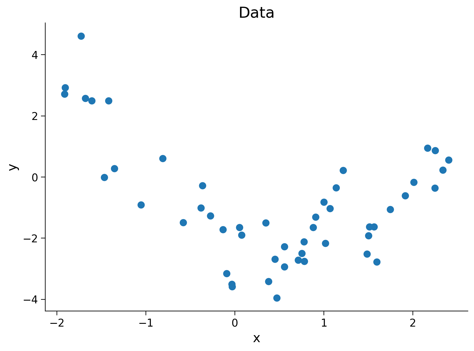
Execute the next cell to generate and plot the data we will fit.
Execute this cell to simulate some data
#@markdown Execute this cell to simulate some data

### Generate training data
np.random.seed(0)
n_train_samples = 50
x_train = np.random.uniform(-2, 2.5, n_train_samples) # sample from a uniform distribution over [-2, 2.5)
noise = np.random.randn(n_train_samples) # sample from a standard normal distribution
y_train =  x_train**2 - x_train - 2 + noise

### Generate testing data
n_test_samples = 20
x_test = np.random.uniform(-3, 3, n_test_samples) # sample from a uniform distribution over [-2, 2.5)
noise = np.random.randn(n_test_samples) # sample from a standard normal distribution
y_test =  x_test**2 - x_test - 2 + noise

## Plot both train and test data
fig, ax = plt.subplots()
plt.title('Data')
plt.plot(x_train, y_train, '.', markersize=15, label='Training')
#plt.plot(x_test, y_test, 'g+', markersize=15, label='Test')
#plt.legend()
plt.xlabel('x')
plt.ylabel('y');
A) Structuring the design matrix#
For linear regression, we used \(X = x\) as our design matrix. To add a constant bias (a y-intercept in a 2-D plot), we use \(X = \big[ \boldsymbol 1, x \big]\), where \(\boldsymbol 1\) is a column of ones. When fitting, we learn a weight for each column of this matrix. So we learn a weight that multiples with column 1 - in this case that column is all ones so we gain the bias parameter (\(+ \theta_0\)). We also learn a weight for every column, or every feature of x.
The key difference between fitting a linear regression model and a polynomial regression model lies in how we create the design matrix. How should we construct the design matrix \(X\) so that a 3rd order polynomial regression model can be in matrix form as \(Y = X\theta\)? What is \(\theta\)? Write out the matrix multiplication for a row of \(Y\) to show it works out equal.
Answer#
Answer here
B) Coding the design matrix#
Complete the function below(make_design_matrix) to structure the design matrix given the input data and the order of the polynomial you wish to fit.
Answer#
Complete code below
def make_design_matrix(x, order):
  """Create the design matrix of inputs for use in polynomial regression

  Args:
    x (ndarray): input vector of shape (n_samples)
    order (scalar): polynomial regression order

  Returns:
    ndarray: design matrix for polynomial regression of shape (samples, order+1)
  """

  # Broadcast to shape (n x 1) so dimensions work
  if x.ndim == 1:
    x = x[:, None]

  #if x has more than one feature, we don't want multiple columns of ones so we assign
  # x^0 here
  design_matrix = np.ones((x.shape[0], 1))

  # Finish creating the design matrix (hint: np.hstack)
  for degree in range(1, order + 1):
      design_matrix = ...

  return design_matrix


order = 5
X_design = make_design_matrix(x_train, order)
print(X_design[0:2, 0:2])
---------------------------------------------------------------------------
TypeError                                 Traceback (most recent call last)
Cell In[5], line 29
     27 order = 5
     28 X_design = make_design_matrix(x_train, order)
---> 29 print(X_design[0:2, 0:2])

TypeError: 'ellipsis' object is not subscriptable
Fitting polynomial regression models#
We will use this design matrix function to fit polynomial regression models of different orders. We are doing this using the same function we completed in Week 9 Tutorial 1 (ordinary_least_squares). I provide you with the code below but just make sure you understand what is happening.
def solve_poly_reg(x, y, order):
  """Fit a polynomial regression model for a given order.

  Args:
    x (ndarray): input vector of shape (n_samples)
    y (ndarray): vector of measurements of shape (n_samples)
    order (scalar): order of polynomial fit

  Returns:
    ndarray: fitted weights of polynomial model
  """

  # Create design matrix
  X_design = make_design_matrix(x, order)

  # Fit polynomial model (use ordinary_least_squares)
  theta_hat = ordinary_least_squares(X_design, y)

  return theta_hat


# Loop over several orders and fit polynomial regressions
max_order = 5
theta_hats = {}
for order in range(max_order + 1):
  theta_hats[order] = solve_poly_reg(x_train, y_train, order)

plot_fitted_polynomials(x_train, y_train, theta_hats)
---------------------------------------------------------------------------
AttributeError                            Traceback (most recent call last)
Cell In[6], line 26
     24 theta_hats = {}
     25 for order in range(max_order + 1):
---> 26   theta_hats[order] = solve_poly_reg(x_train, y_train, order)
     28 plot_fitted_polynomials(x_train, y_train, theta_hats)

Cell In[6], line 17, in solve_poly_reg(x, y, order)
     14 X_design = make_design_matrix(x, order)
     16 # Fit polynomial model (use ordinary_least_squares)
---> 17 theta_hat = ordinary_least_squares(X_design, y)
     19 return theta_hat

Cell In[3], line 15, in ordinary_least_squares(X, y)
      4 """Ordinary least squares estimator for linear regression.
      5
      6 Args:
   (...)
     11   ndarray: estimated parameter values of shape (n_regressors)
     12 """
     14 # Compute theta_hat using OLS
---> 15 theta_hat = np.linalg.inv(X.T @ X) @ X.T @ y
     17 return theta_hat

AttributeError: 'ellipsis' object has no attribute 'T'
In this exercise, we saw we could create a polynomial regression model by using the linear regression setup and altering the design matrix. Altering the design matrix and using linear regression is a powerful tool! For example, in neuroscience, we might want to fit temporal lags (so recent history of a stimulus, not just the current frame). We can create the design matrix in such a way as to include the temporal lags
Exercise 2: Bias variance tradeoff#
A) Thinking about models#
Answer these before moving on
These questions relate to the models we’ve just fit in Exercise 1:
i) Which model do you think will have the lowest training MSE (mean squared error on the data with which the models are fit)? Why?
ii) Which model do you think could have lowest test MSE? Why? (we’ll accept several answers as long as the reasoning is good since it’s hard to tell from the plot)
iii) Which model has lowest variance (and highest bias)? Why?
iv) Which model has high variance and low bias? Why?
Now look at the next sections to validate your answers.
Answer#
Answer here
Looking at bias vs variance#
In the plots below, I have resampled new data sets (new samples) from the true data distribution. I have fit each polynomial order to each new sample. Note that we cannot usually resample data from the actual distribution - we would normally use bootstrapping!
I am plotting the true data model in black and each fit model in green.
Execute to visualize multiple fits
# @markdown Execute to visualize multiple fits
np.random.seed(121)

fig, axes = plt.subplots(1, 6, figsize = (15, 4), sharey=True)


x_grid = np.linspace(x_train.min() - .5, x_train.max() + .5)
X_design = {}
y_hats = {}
for order in range(max_order + 1):
  X_design[order] = make_design_matrix(x_grid, order)
  y_hats[order] = np.zeros((0, len(x_grid)))

for i_sample in range(30):

  # Sample new data
  n_samples = 30
  x = np.random.uniform(-2, 2.5, n_samples)  # inputs uniformly sampled from [-2, 2.5)
  y =  x**2 - x - 2   # computing the outputs

  output_noise = 1.5 * np.random.randn(n_samples)
  y += output_noise  # adding some output noise

  # Loop over several orders and fit polynomial regressions
  max_order = 5
  theta_hats = {}
  for order in range(max_order + 1):
    theta_hats[order] = solve_poly_reg(x, y, order)

    y_hat = X_design[order] @ theta_hats[order]
    y_hats[order] = np.concatenate((y_hats[order], y_hat[None, :]), axis=0)
    axes[order].plot(x_grid, y_hat, 'g', alpha=.2, label='Fitted models' if i_sample == 0 else "")

for order in range(max_order + 1):
  axes[order].plot(x_grid, X_design[2] @ np.array([-2, -1, 1]), 'k', label='True model')
  axes[order].set(ylim=[-15, 15], xlabel='x', ylabel='y', title='Order '+str(order))

leg = axes[0].legend(loc='best', frameon=False, handlelength=0)
# change the font colors to match the line colors:
for line,text in zip(leg.get_lines(), leg.get_texts()):
    text.set_color(line.get_color())
---------------------------------------------------------------------------
AttributeError                            Traceback (most recent call last)
Cell In[7], line 28
     26 theta_hats = {}
     27 for order in range(max_order + 1):
---> 28   theta_hats[order] = solve_poly_reg(x, y, order)
     30   y_hat = X_design[order] @ theta_hats[order]
     31   y_hats[order] = np.concatenate((y_hats[order], y_hat[None, :]), axis=0)

Cell In[6], line 17, in solve_poly_reg(x, y, order)
     14 X_design = make_design_matrix(x, order)
     16 # Fit polynomial model (use ordinary_least_squares)
---> 17 theta_hat = ordinary_least_squares(X_design, y)
     19 return theta_hat

Cell In[3], line 15, in ordinary_least_squares(X, y)
      4 """Ordinary least squares estimator for linear regression.
      5
      6 Args:
   (...)
     11   ndarray: estimated parameter values of shape (n_regressors)
     12 """
     14 # Compute theta_hat using OLS
---> 15 theta_hat = np.linalg.inv(X.T @ X) @ X.T @ y
     17 return theta_hat

AttributeError: 'ellipsis' object has no attribute 'T'
We can see that the order 5 model fits vary a lot based on the sample of data used - there is a lot of variance over different data samples. On average though, these fits resemble the true model (if you average over the green lines, it is roughly the black line) so this model has low bias. The order 0 model has high bias since the predictions do not match the true model on average (but lower variance than the order 5 model). By eye, the order 2 model looks about right as a balance between these tendencies.
Looking at train vs test MSE#
We can compute the mean squared error of each polynomial model on the data it is fit with (the training data) and held-out data (the test data). No need to answer this explicitly here but discuss how the training MSE should change over order and how the test MSE should before seeing the plot.
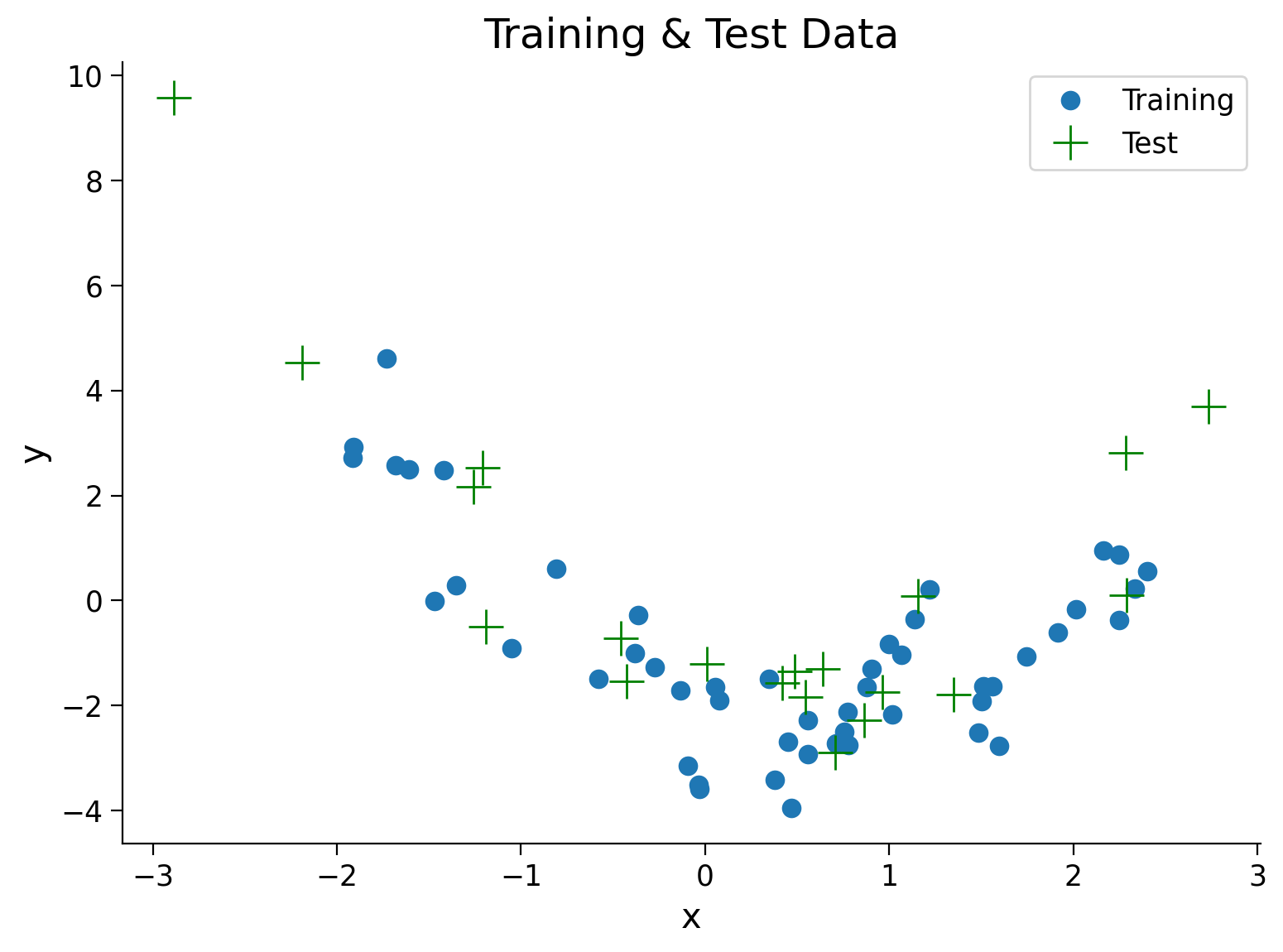
Execute to see train and test data
# @markdown Execute to see train and test data
## Plot both train and test data
fig, ax = plt.subplots()
plt.title('Training & Test Data')
plt.plot(x_train, y_train, '.', markersize=15, label='Training')
plt.plot(x_test, y_test, 'g+', markersize=15, label='Test')
plt.legend()
plt.xlabel('x')
plt.ylabel('y');
Execute to see train vs test MSE
# @markdown Execute to see train vs test MSE
mse_train = np.zeros((max_order+1))
mse_test = np.zeros((max_order+1))
for order in range(max_order + 1):
  theta_hat = solve_poly_reg(x_train, y_train, order)
  mse_train[order] = evaluate_poly_reg(x_train, y_train, theta_hat, order)
  mse_test[order] = evaluate_poly_reg(x_test, y_test, theta_hat, order)

fig, ax = plt.subplots()
width = .35

ax.bar(np.arange(max_order + 1) - width / 2, mse_train, width, label="train MSE")
ax.bar(np.arange(max_order + 1) + width / 2, mse_test , width, label="test MSE")

ax.legend()
ax.set(xlabel='Polynomial order', ylabel='MSE', title ='Comparing polynomial fits');
---------------------------------------------------------------------------
AttributeError                            Traceback (most recent call last)
Cell In[9], line 5
      3 mse_test = np.zeros((max_order+1))
      4 for order in range(max_order + 1):
----> 5   theta_hat = solve_poly_reg(x_train, y_train, order)
      6   mse_train[order] = evaluate_poly_reg(x_train, y_train, theta_hat, order)
      7   mse_test[order] = evaluate_poly_reg(x_test, y_test, theta_hat, order)

Cell In[6], line 17, in solve_poly_reg(x, y, order)
     14 X_design = make_design_matrix(x, order)
     16 # Fit polynomial model (use ordinary_least_squares)
---> 17 theta_hat = ordinary_least_squares(X_design, y)
     19 return theta_hat

Cell In[3], line 15, in ordinary_least_squares(X, y)
      4 """Ordinary least squares estimator for linear regression.
      5
      6 Args:
   (...)
     11   ndarray: estimated parameter values of shape (n_regressors)
     12 """
     14 # Compute theta_hat using OLS
---> 15 theta_hat = np.linalg.inv(X.T @ X) @ X.T @ y
     17 return theta_hat

AttributeError: 'ellipsis' object has no attribute 'T'
Exercise 3: Model selection via cross validation#
In Exercise 2, we sampled multiple times from the actual distribution and looked at the test data to think about best model fits - neither of which we can usually do! Let’s do model selection properly using cross-validation.
A) By hand implementation on a toy example#
We usually use sklearn for cross-validation in python. We will first implement cross-validation for a tiny toy example to make sure we understand the steps.
Let’s say we have:
We want to fit the model: $\(y = \theta\)\( The least squares solution (see derivation below) is \)\(\hat{\theta} = \frac{\sum y_i}{N}\)$
Note that this is a standard baseline model - we are essentially modeling y as the average of y in the training data. This would be like predicting the responses of a neuron by using the mean firing rate.
Use 3 fold cross validation (by hand) and report the validation MSE for this model on this data. You may use code or do this by hand, but don’t use any functions for cross validation. Show your work (i.e. specify how you’re splitting the data, report the validation MSE for every split, etc).
Answer#
Answer here
We could do the same procedure for \(y = \theta x\) and use the validation MSE to pick which model is better (telling us whether y is at all correlated with x). We won’t though for time!
Derivation of least squares solution $\(\begin{align} y &= \theta \\ MSE & = \frac{1}{N} \sum_i (y_i - \hat{y}_i)^2 \\ & = \frac{1}{N} \sum_i (y_i - \theta)^2 \\ \frac{dMSE}{d\theta} &= \frac{2}{N} \sum_i (y_i - \theta) \\ &= \sum_i (y_i - \theta) \\ &= \sum_i y_i - \sum_i \theta \\ &= \sum_i y_i - N\theta = 0 \\ \hat{\theta} &= \frac{\sum_i y_i}{N} \end{align}\)$
B) Using sklearn#
Now we can use sklearn to perform cross-validation and select the our model from the different order polynomial models. Here I just use sklearn to get the train/val splits (using the Kfold iterator) and then use our functions above to fit the models. At the end of this tutorial, I show how to do everything (including fitting the models) in sklearn.
Nothing to do here but look at the plot and answer the question - I show you the code in case you want to look through it.
from sklearn.model_selection import KFold

def cross_validate(x_train, y_train, max_order, n_splits):
  """ Compute MSE for k-fold validation for each order polynomial

  Args:
    x_train (ndarray): training data input vector of shape (n_samples)
    y_train (ndarray): training vector of measurements of shape (n_samples)
    max_order (scalar): max order of polynomial fit
    n_split (scalar): number of folds for k-fold validation

  Return:
    ndarray: MSE over splits for each model order, shape (n_splits, max_order + 1)

  """
  # Initialize the split method
  kfold_iterator = KFold(n_splits)

  # Initialize np array mse values for all models for each split
  mse_all = np.zeros((n_splits, max_order + 1))

  for i_split, (train_indices, val_indices) in enumerate(kfold_iterator.split(x_train)):

      # Split up the overall training data into cross-validation training and validation sets
      x_cv_train = x_train[train_indices]
      y_cv_train = y_train[train_indices]
      x_cv_val = x_train[val_indices]
      y_cv_val = y_train[val_indices]

      # Fit and evaluate models
      for order in range(max_order + 1):
          theta_hat = solve_poly_reg(x_cv_train, y_cv_train, order)
          mse_all[i_split, order] = evaluate_poly_reg(x_cv_val, y_cv_val, theta_hat, order)

  return mse_all


# Call function and plot
max_order = 5
n_splits = 10

plt.figure()

mse_all = cross_validate(x_train, y_train, max_order, n_splits)
plt.boxplot(mse_all, labels=np.arange(0, max_order + 1))

plt.xlabel('Polynomial Order')
plt.ylabel('Validation MSE')
plt.title(f'Validation MSE over {n_splits} splits of the data');
---------------------------------------------------------------------------
ModuleNotFoundError                       Traceback (most recent call last)
Cell In[10], line 1
----> 1 from sklearn.model_selection import KFold
      3 def cross_validate(x_train, y_train, max_order, n_splits):
      4   """ Compute MSE for k-fold validation for each order polynomial
      5
      6   Args:
   (...)
     14
     15   """

ModuleNotFoundError: No module named 'sklearn'
Which polynomial order do you think is a better model of the data based on cross-validation? Why?
Note it may not be what you expected - we’ll discuss in class!
Answer#
Answer here
Coding Fun: Everything in sklearn#
Let’s look at implementing polynomial regression models, fitting them, and performing cross-validation entirely in sklearn.
We create a polynomial regression model by chaining together a preprocessing step that turns the data into polynomial features and a linear regression model. (Note that if we have more than 1D data, this would create interaction terms which we may not want).
See here for more details: https://towardsdatascience.com/polynomial-regression-with-scikit-learn-what-you-should-know-bed9d3296f2
The code below fits an order 3 polynomial regression model, looks at the fitted parameters, and gets predictions/R2 value
from sklearn.preprocessing import PolynomialFeatures
from sklearn.pipeline import make_pipeline
from sklearn.linear_model import LinearRegression

# Create polynomial regression model
degree = 3
poly_reg = make_pipeline(PolynomialFeatures(degree),LinearRegression())

# Fit this model to data
poly_reg.fit(x_train[:, None], y_train)

# You can now look at theta_hat
print(poly_reg['linearregression'].coef_)

# Let's make predictions on test data
y_hat = poly_reg.predict(x_test[:, None])

# Let's evaluate on test data (this returns R2)
poly_reg.score(x_test[:, None], y_test)
---------------------------------------------------------------------------
ModuleNotFoundError                       Traceback (most recent call last)
Cell In[11], line 1
----> 1 from sklearn.preprocessing import PolynomialFeatures
      2 from sklearn.pipeline import make_pipeline
      3 from sklearn.linear_model import LinearRegression

ModuleNotFoundError: No module named 'sklearn'
The code below does cross validation with 10 splits for an order 3 polynomial regression model. We could loop over this to get the validation MSE for each order model.
from sklearn.model_selection import cross_val_score

## Let's get validation MSE for this model using cross-validation

# Create polynomial regression model
degree = 3
poly_reg = make_pipeline(PolynomialFeatures(degree),LinearRegression())

# Cross-validation
val_mse = cross_val_score(poly_reg, x_train[:, None], y_train, cv = 10, scoring='neg_mean_squared_error')

# This has return negative MSE so let's get actual MSE
val_mse *= -1

print(val_mse)
---------------------------------------------------------------------------
ModuleNotFoundError                       Traceback (most recent call last)
Cell In[12], line 1
----> 1 from sklearn.model_selection import cross_val_score
      3 ## Let's get validation MSE for this model using cross-validation
      4
      5 # Create polynomial regression model
      6 degree = 3

ModuleNotFoundError: No module named 'sklearn'
Let’s get really fancy and using GridSearchCV to search over all the orders of polynomial regression we’re looking at and perform cross-validation for each.
from sklearn.model_selection import GridSearchCV

# Parameters we want to search over
parameters = {'polynomialfeatures__degree': [0, 1, 2, 3, 4, 5]}

# Set up cross validation
poly_reg = make_pipeline(PolynomialFeatures(),LinearRegression())

cv = GridSearchCV(poly_reg, parameters, cv = 10, scoring='neg_mean_squared_error')
cv.fit(x_train[:, None], y_train)

plt.plot(np.arange(max_order + 1), -1*cv.cv_results_['mean_test_score'], '-og')
plt.xlabel('Order')
plt.ylabel('Validation MSE');
---------------------------------------------------------------------------
ModuleNotFoundError                       Traceback (most recent call last)
Cell In[13], line 1
----> 1 from sklearn.model_selection import GridSearchCV
      3 # Parameters we want to search over
      4 parameters = {'polynomialfeatures__degree': [0, 1, 2, 3, 4, 5]}

ModuleNotFoundError: No module named 'sklearn'