Tutorial 2

[insert your name]

Please note: this is an unusual tutorial - there are no exercises and you do not need to submit it! Please read through and engage with the material/demos though.

Imports

# @markdown Imports

# Imports
import numpy as np
import matplotlib.pyplot as plt
import ipywidgets as widgets  # interactive display
import scipy.io

Plotting functions

# @markdown Plotting functions
import numpy
from numpy.linalg import inv, eig
from math import ceil
from matplotlib import pyplot, ticker, get_backend, rc
from mpl_toolkits.mplot3d import Axes3D
from itertools import cycle


%config InlineBackend.figure_format = 'retina'
plt.style.use("https://raw.githubusercontent.com/NeuromatchAcademy/course-content/master/nma.mplstyle")

classic = 'k'

Using SVD for Receptive Field Exploration

Execute this cell to generate a receptive field

# @markdown Execute this cell to generate a receptive field

np.random.seed(123)

def twoD_Gaussian(xdata_tuple, amplitude, xo, yo, sigma_x, sigma_y, theta, offset):
    (x, y) = xdata_tuple
    xo = float(xo)
    yo = float(yo)    
    a = (np.cos(theta)**2)/(2*sigma_x**2) + (np.sin(theta)**2)/(2*sigma_y**2)
    b = -(np.sin(2*theta))/(4*sigma_x**2) + (np.sin(2*theta))/(4*sigma_y**2)
    c = (np.sin(theta)**2)/(2*sigma_x**2) + (np.cos(theta)**2)/(2*sigma_y**2)
    g = offset + amplitude*np.exp( - (a*((x-xo)**2) + 2*b*(x-xo)*(y-yo)+c*((y-yo)**2)))
    return g.ravel()


x = np.arange(0, 20, 1)
y = np.arange(0, 20, 1)
x, y = np.meshgrid(x, y)

STA_temporal = np.array([ 0.01,  0.  ,  0.  , -0.01, -0.01, -0.02, -0.03, -0.04, -0.05,
       -0.07, -0.08, -0.09, -0.08, -0.03,  0.09,  0.28,  0.47,  0.56,
        0.5 ,  0.33,  0.16,  0.05,  0.  , -0.01, -0.01])

sd_x = 2 
sd_y = 2
gauss = twoD_Gaussian((x,y), 1, 6, 10, sd_x, sd_y, 0, 0)
STA_spatial = gauss.reshape((20,20))
STA_spatial[STA_spatial<.05]=0
full_STA = np.outer(STA_temporal, STA_spatial).reshape((-1, 20, 20))
full_STA += .01*np.random.randn(full_STA.shape[0], full_STA.shape[1], full_STA.shape[2])
full_STA -= np.mean(full_STA)
STA_spatial += .01*np.random.randn(STA_spatial.shape[0], STA_spatial.shape[1])

A spatiotemporal receptive field

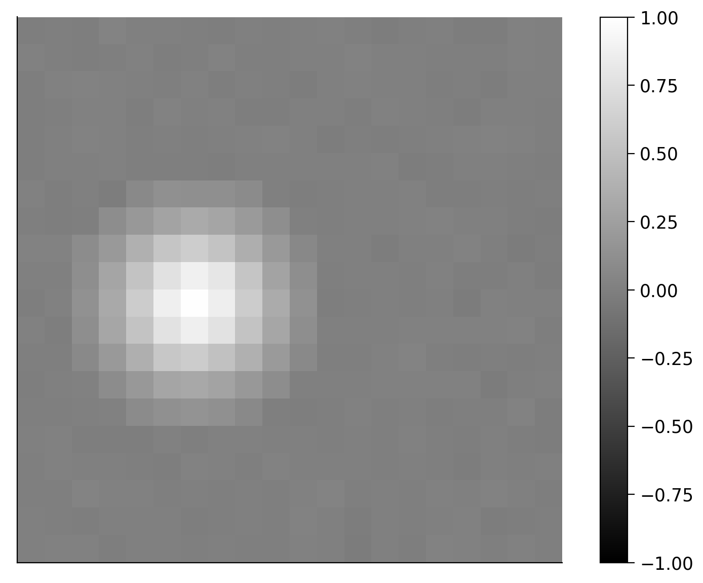
Let’s say we are recording the activity of a retinal neuron in response to a visual stimulus. We have estimated its receptive field using an analysis such as spike-triggered average. Don’t worry if you’re not familiar with spike-triggered averages - the point here is just that we have some estimate of the neurons receptive field.

This retinal neuron responds to light patterns in a certain part of the visual field (space). If there was no temporal component to the response, the receptive field might look like that shown below where the space is represented by a 20 x 20 pixel image. We can see from this receptive field that the neuron respond more when light pixels are present in the left middle region of the image.

Note: the receptive fields shown in this tutorial are simulated for ease of visualization but based pretty closely on real retinal neuron receptive fields.

Execute to visualize spatial receptive field

# @markdown Execute to visualize spatial receptive field
fig, ax = plt.subplots()
im = ax.imshow(STA_spatial,vmin=-1, vmax=1,  cmap='gray')
ax.set(xticks=[], yticks=[]);
plt.colorbar(im);

This retinal neuron does have a temporal component to the response though because its response depends on the very recent history of the visual stimulus. Note that this is true of almost all neurons, if not all! We want to know how the image 140 milliseconds (ms) ago affects responses vs the image 80 ms ago, and so on. So we look at the spatial receptive field at each of those time points, as shown below.

Execute this cell to visualize spatial receptive field at two time points

# @markdown Execute this cell to visualize spatial receptive field at two time points
fig, (ax, ax2, cax) = plt.subplots(ncols=3,figsize=(7,3), 
                  gridspec_kw={"width_ratios":[1,1, 0.05]})
fig.subplots_adjust(wspace=0.3)
im = ax.imshow(full_STA[11], vmin=-.6, vmax=.6, cmap='gray')
ax.set(xticks=[], yticks=[], title='140 ms ago');
im = ax2.imshow(full_STA[17], vmin=-.6, vmax=.6, cmap='gray')
ax2.set(xticks=[], yticks=[], title='80 ms ago');

fig.colorbar(im, cax=cax);

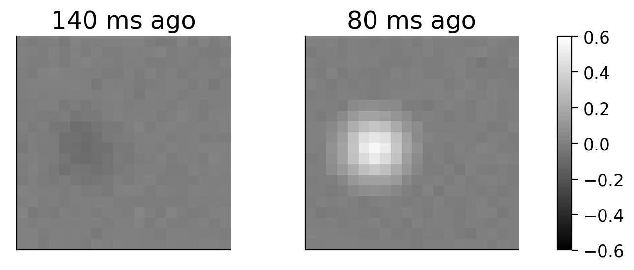
You can see that the spatial receptive field looks quite different at each of these time points! In fact, it’s basicaly the reverse - the neuron responds more to dark pixels in that region 140 ms before and light pixels in that region 80 ms before.

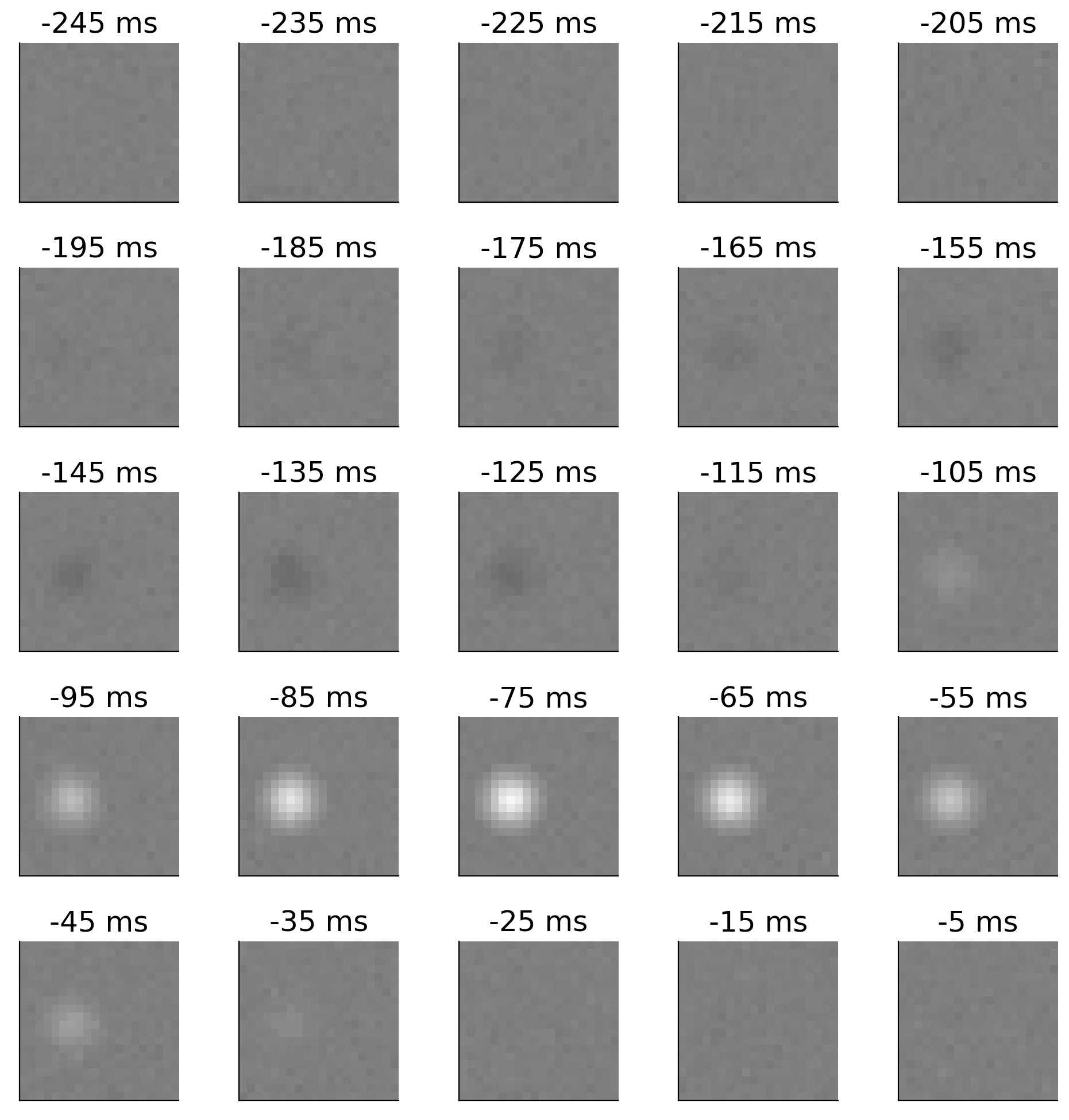
So, we need a spatiotemporal receptive field of the neuron. It’s too difficult to model the spatial receptive field at every single time point in recent history because there are an infinite amount of those (40.1 ms ago, 40.211 ms ago, etc). Instead, we bin time and estimate the spatial receptive field for that small span of time. In this case, we will bin time into 10 ms bins. So we have the spatial receptive field from 10-0 ms ago, 20-10 ms ago, 30-20 ms ago, etc. For this retinal neuron, the size of our receptive field is 25 x 20 x 20, where the first dimension (25) is the temporal component and corresponds to 10 ms bins. So we’re modeling the receptive field 25 bins x 10 ms/bin = 250 ms back in time. We can refer to the 10 ms bins as frames of our spatiotemporal field as they are like frames of a movie.

The next plot shows this receptive field - we have 25 frames of the spatial receptive field.

Execute this cell to visulize all 25 frames

# @markdown Execute this cell to visulize all 25 frames
frame_stamps = np.arange(5, 25*10, 10)[::-1]
fig, axes = plt.subplots(5, 5, figsize=(10,10))

row=0
col=0
for i_frame in range(25):
    axes[row][col].imshow(full_STA[i_frame], vmin=-.6, vmax=.6, cmap='gray')
    axes[row][col].set(xticks=[], yticks=[], title='-' + str(frame_stamps[i_frame]) + ' ms')
    
    col+=1
    if col==5:
        col=0
        row+=1

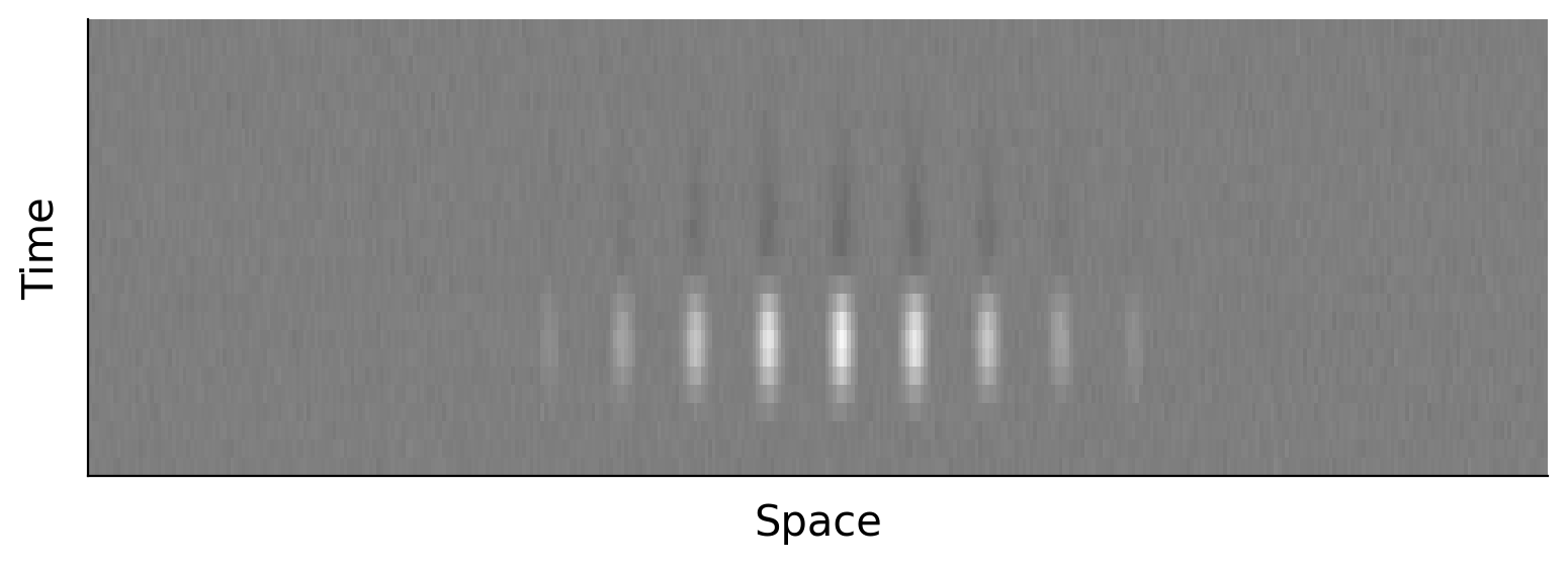
We will often flatten the spatial component of the receptive field for ease of analysis so we would then have a 30 x 1600 receptive field.

Execute this cell to visualize flattened receptive field

# @markdown Execute this cell to visualize flattened receptive field

fig, ax = plt.subplots()
ax.imshow(full_STA.reshape((25, -1)), vmin=-0.6, vmax=.6, cmap='gray')
ax.set(xticks=[], yticks=[], xlabel='Space', ylabel='Time');
ax.set_aspect(5)

Parsing a separable spatiotemporal receptive field

In the plot above, we can see that the spatial receptive field is not widely different at every frame. There is some consistency to it over time. It seems like there might be a better way to understand the receptive field of this neuron than looking at all 25x20x20= 10,000 pixels of the spatiotemporal receptive field. In fact, it is possible that we can well approximate the full spatiotemporal receptive field as the same spatial receptive field that is just weighted differently at every point in time. This would mean we could summarize the full receptive field with just a single spatial filter and a temporal filter (which tells us the weighting of the spatial filter at each point in time). This means the receptive field is separable (into space and time).

See the demo below

Execute this cell to enable demo

# @markdown Execute this cell to enable demo
from matplotlib.patches import Rectangle

def plot_filters(t):
    fig, axes = plt.subplots(1, 3, figsize=(20,5))
    axes[0].plot(frame_stamps[::-1], STA_temporal,'-ok')
    axes[0].set(title='Temporal filter', xlabel='Time before present (ms)', xticks=frame_stamps[::-2], xticklabels=frame_stamps[::2])
    axes[1].imshow(STA_spatial, vmin=-.6, vmax=.6,cmap='gray')
    axes[1].set(title='Standard Spatial filter', xticks=[], yticks=[]);
    axes[0].set_xlim([0, 250])
    axes[0].add_patch(Rectangle((245-t, -.1), 10, .66, color='r', fill=None, alpha=1, linewidth=2))

    axes[2].imshow(STA_spatial*STA_temporal[np.where(frame_stamps==t)[0]], vmin=-.6, vmax=.6, cmap='gray')
    axes[2].set(title='Spatial RF at '+str(t)+'ms ago', xticks=[], yticks=[]);
    axes[0].annotate('x', (.37, .5), xycoords='figure fraction', color='r', fontsize=50)
    axes[2].annotate('=', (.7, .5), xycoords='figure fraction', color='r', fontsize=50)

_ = widgets.interact(plot_filters, t=(5, 245, 10))

How do we find this temporal filter and spatial filter though? Let’s first answer the opposite question: how would we form a full spatiotemporal filter from these two filters?

Let’s flatten the spatial filter so now the temporal filter has 25 entries and the spatial filter has 400 entries (20 x 20). It turns out that we could reconstruct the full spatiotemporal receptive field from the outer product of these two vectors! This is the definition of an outer product - refer to Video 5.2 at 18:12 to review this.

Hmm, we’ve heard before about forming a matrix as the outer product of two vectors… That’s what we do when we form a low rank approximation of a matrix using SVD. Recall that the SVD of a matrix is:

\[ X = USV^T\]

It factorizes the matrix X into the product of three matrices where U and V are orthogonal and S is a diagonal matrix. We can view this slightly differently: SVD factorizes a matrix into a sum of outer products of decreasing influence. So:

\[ X = s_1\bar{u}_1\bar{v}_1^T + s_2\bar{u}_2\bar{v}_2^T + s_3\bar{u}_3\bar{v}_t^T + ... \]

We can take the first k terms of this sum and reconstruct a rank k approximation of X. Let’s just take the first term:

\[ X = s_1\bar{u}_1\bar{v}_1^T \]

We can see that we’re reconstructing the matrix X as an outer product of two vectors (\(\bar{u}_1\) and \(\bar{v}_1\)), multiplied by scalar \(s_1\).

So, if we want to reconstruct a matrix as the outer product of two vectors, SVD gives us the best possible vectors to do that: the two vectors that will get us as close to our original matrix as possible. We can use this fact to find our temporal and spatial receptive field from our full spatiotemporal receptive field: perform SVD on the full spatiotemporal receptive field and the first column of U is the temporal filter and the first column of V is the spatial filter. Let’s see this done in the code below.

full_STA.shape

(25, 20, 20)

U, s, VT = np.linalg.svd(full_STA.reshape((25, -1)))
temporal_filter = U[:, 0]
spatial_filter = VT.T[:, 0].reshape((20, 20))

Execute to visualize filters

# @markdown Execute to visualize filters
# Plot filters
fig, axes = plt.subplots(1, 2, figsize=(20,5))
axes[0].plot(frame_stamps[::-1], temporal_filter,'k')
axes[0].set(title='Temporal filter', xlabel='Time before present (ms)', xticks=frame_stamps[::-2], xticklabels=frame_stamps[::2])
axes[1].imshow(spatial_filter, cmap='gray')
axes[1].set(title='Spatial filter', xticks=[], yticks=[]);

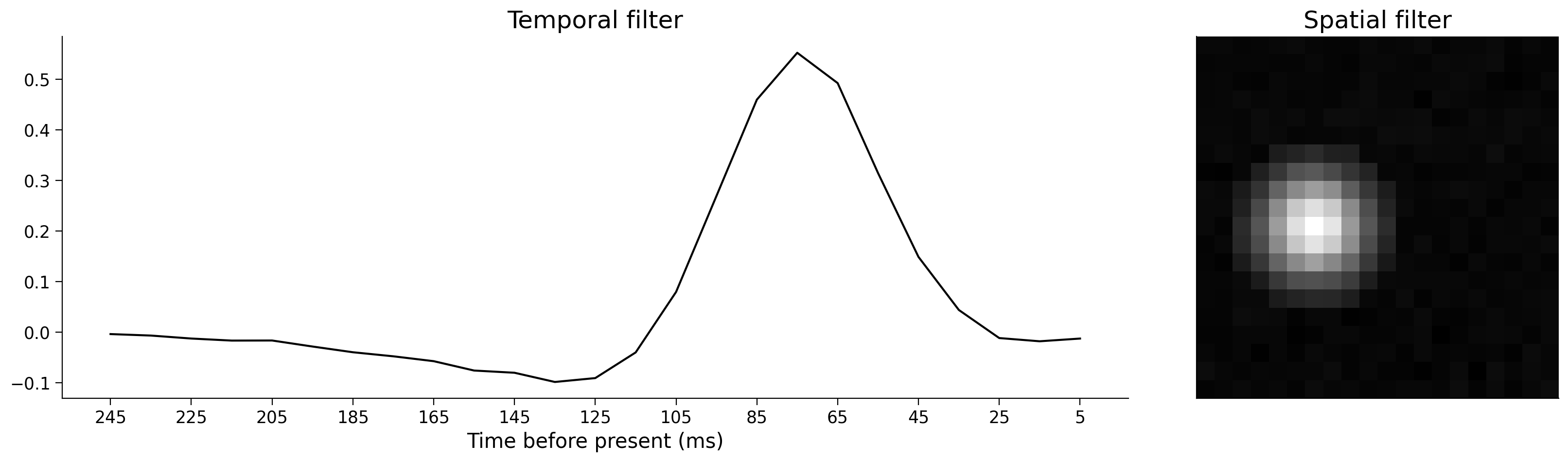
Note that we start to understand the neural processing more easily than using the full spatiotemporal receptive field above as these filters are far more condensed. We know how the neuron responds over time and over space separately. We can easily tell what the lag is from peak stimulus drive to response (~70 ms).

Assessing separability

In the above example, I told you that the spatiotemporal receptive field was separable - it could be well described by a single temporal receptive field and spatial temporal field. How could you have known this for yourself?

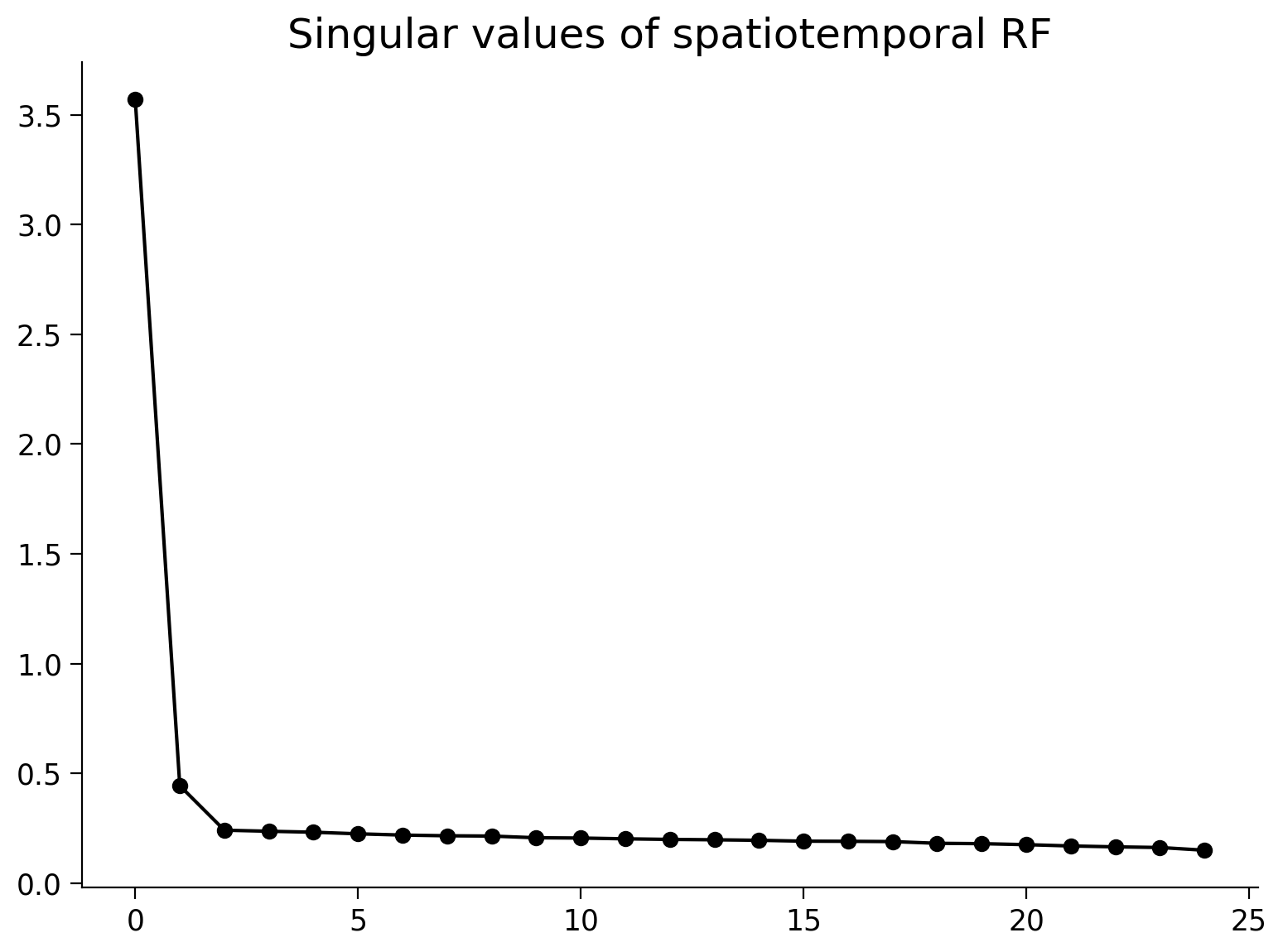
You can look at the singular values (the entries of S). If the matrix is perfectly reconstructed as an outer product of two vectors, only the first singular value will be non-zero. In practice, this will never be the case with receptive fields as there will be some noise so you will not be able to perfectly reconstruct with just two vectors and the the first singular value will not be the only non-zero one. However, you can still look at the values of the singular values to assess separability: if the first singular value is far higher than the rest, the receptive field is pretty well approximated by a single temporal filter and a single spatial receptive field. You can validate from the plot below that this is the case with the receptive field we’ve been working with.

Execute to visualize singular values

# @markdown Execute to visualize singular values
fig, ax = plt.subplots()
ax.plot(s, '-ok')
ax.set(title='Singular values of spatiotemporal RF');

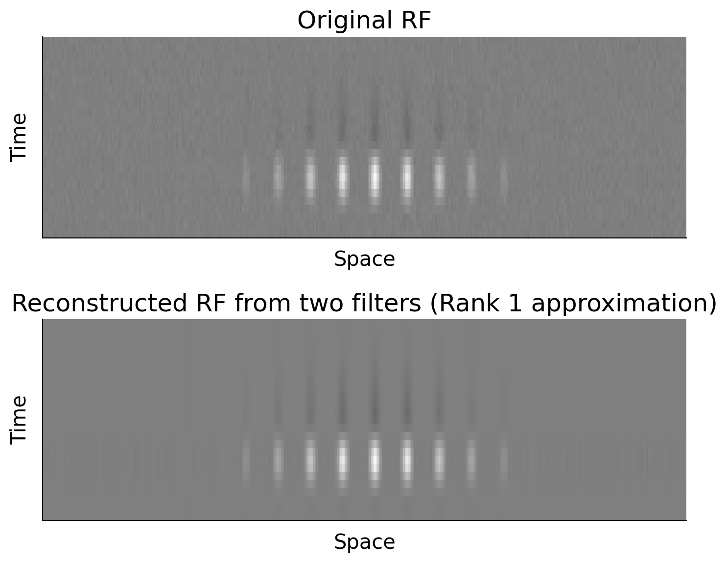
It’s of course always good to check that your reconstructed spatiotemporal filter looks reasonably close to the original one. You could even compute some sort of similarity metric, such as mean squared error (we’ll get to this later in the course!). You can see that the reconstructed rank 1 approximation has gotten rid of some of the noise present in the original receptive field

Execute this cell to visualize original vs rank 1 approximation

# @markdown Execute this cell to visualize original vs rank 1 approximation
spatiotemporal_STA = s[0]*np.outer(temporal_filter, spatial_filter.reshape((-1,)))

fig, axes = plt.subplots(2, 1)
axes[0].imshow(full_STA.reshape((25, -1)), vmin=-0.6, vmax=.6, cmap='gray')
axes[0].set(xticks=[], yticks=[], xlabel='Space', ylabel='Time', title='Original RF');
axes[0].set_aspect(5)
axes[1].imshow(spatiotemporal_STA.reshape((25, -1)), vmin=-0.6, vmax=.6, cmap='gray')
axes[1].set(xticks=[], yticks=[], xlabel='Space', ylabel='Time', title='Reconstructed RF from two filters (Rank 1 approximation)');
axes[1].set_aspect(5)

Multiple temporal & spatial filters

Sometimes, a spatiotemporal receptive field won’t be fully separable but SVD can still be useful. The receptive field may not be well described by a single spatial filter and a single temporal filter but could be approximated well by a rank 2 approximation. This means that we’d take the first 2 terms of the sum of outer products from the singular value decomposition. The full spatiotemporal receptive field is equivalent to adding two separable spatiotemporal receptive fields. We’d end up with two temporal filters and two spatial filters.

The implications of this for the neural processing are interesting. For example, you could imagine that this may be a neuron that gets inputs from two neurons with separable receptive fields. This is not the only explanation though!

Moving beyond space and time

We have used the example of a spatiotemporal receptive field and using SVD to find a temporal filter and a spatial filter. Note that this is not the only case in which you can use SVD to parse the receptive field, just the most obvious/most intuitive one. Anytime you have a receptive field formed from two different types of information (time vs space in this case), you can use this method to assess the separability of the receptive field into two distinct filters that each operate on one of the types of information. As a perhaps silly example, you could have a receptive field of a neuron in actual space based on the animals position (like for a place cell) where the two types of information are two axes of space (north-south, east-west). You could determine whether this receptive field is separable, meaning that the neuron has a single east-west filter and a single north-south filter and the neuron responds as the sum of the activation of each of these filters.

More resources

A great blog post on this topic: https://xcorr.net/2011/09/20/using-the-svd-to-estimate-receptive-fields/

A paper that looks at the separability of receptive fields: https://www.pnas.org/content/99/3/1645.full

Another paper that uses SVD on receptive fields: https://www.cambridge.org/core/journals/visual-neuroscience/article/temporal-diversity-in-the-lateral-geniculate-nucleus-of-cat/8FBDFA2D271BE6E48537ACDD485F29FB

Whitening before PCA

You may sometimes want to whiten your data before applying PCA. This is an option in sklearn.decomposition.PCA. From their docs: “the component vectors are multiplied by the square root of n_samples and then divided by the singular values to ensure uncorrelated outputs with unit component-wise variances. Whitening will remove some information from the transformed signal (the relative variance scales of the components) but can sometime improve the predictive accuracy of the downstream estimators by making their data respect some hard-wired assumptions.” https://scikit-learn.org/stable/modules/generated/sklearn.decomposition.PCA.html

We will be addressing whitening in the machine learning section of this course but just wanted to put this on your radar in case you use PCA before then.