Tutorial 2

Probability & Statistics II: Intro to Statistics

[insert your name]

Important reminders: Before starting, click “File -> Save a copy in Drive”. Produce a pdf for submission by “File -> Print” and then choose “Save to PDF”.

To complete this tutorial, you should have watched Videos 7.1 - 7.4

Imports

# @markdown Imports

# Imports

import numpy as np
import matplotlib.pyplot as plt
import ipywidgets as widgets  # interactive display
import math

Plotting functions

# @markdown Plotting functions
import numpy
from numpy.linalg import inv, eig
from math import ceil
from matplotlib import pyplot, ticker, get_backend, rc
from mpl_toolkits.mplot3d import Axes3D
from itertools import cycle
from IPython.display import clear_output
from ipywidgets import FloatSlider, Dropdown, interactive_output
from ipywidgets import interact, fixed, HBox, Layout, VBox, interactive, Label


%config InlineBackend.figure_format = 'retina'
plt.style.use("https://raw.githubusercontent.com/NeuromatchAcademy/course-content/master/nma.mplstyle")

def plot_mixture_prior(x, gaussian1, gaussian2, combined):
    """ Plots a prior made of a mixture of gaussians

    Args:
      x (numpy array of floats):         points at which the likelihood has been evaluated
      gaussian1 (numpy array of floats): normalized probabilities for Gaussian 1 evaluated at each `x`
      gaussian2 (numpy array of floats): normalized probabilities for Gaussian 2 evaluated at each `x`
      posterior (numpy array of floats): normalized probabilities for the posterior evaluated at each `x`

    Returns:
      Nothing
    """
    fig, ax = plt.subplots()
    ax.plot(x, gaussian1, '--b', LineWidth=2, label='Gaussian 1')
    ax.plot(x, gaussian2, '-.b', LineWidth=2, label='Gaussian 2')
    ax.plot(x, combined, '-r', LineWidth=2, label='Gaussian Mixture')
    ax.legend()
    ax.set_ylabel('Probability')
    ax.set_xlabel('Orientation (Degrees)')


def plot_gaussian(μ, σ):
    x = np.linspace(-7, 7, 1000, endpoint=True)
    y = gaussian(x, μ, σ)

    plt.figure(figsize=(6, 4))
    plt.plot(x, y, c='blue')
    plt.fill_between(x, y, color='b', alpha=0.2)
    plt.ylabel('$\mathcal{N}(x, \mu, \sigma^2)$')
    plt.xlabel('x')
    plt.yticks([])
    plt.show()


def plot_losses(μ, σ):
    x = np.linspace(-2, 2, 400, endpoint=True)
    y = gaussian(x, μ, σ)
    error = x - μ

    mse_loss = (error)**2
    abs_loss = np.abs(error)
    zero_one_loss = (np.abs(error) >= 0.02).astype(np.float)

    fig, (ax_gaus, ax_error) = plt.subplots(2, 1, figsize=(6, 8))
    ax_gaus.plot(x, y, color='blue', label='true distribution')
    ax_gaus.fill_between(x, y, color='blue', alpha=0.2)
    ax_gaus.set_ylabel('$\\mathcal{N}(x, \\mu, \\sigma^2)$')
    ax_gaus.set_xlabel('x')
    ax_gaus.set_yticks([])
    ax_gaus.legend(loc='upper right')

    ax_error.plot(x, mse_loss, color='c', label='Mean Squared Error', linewidth=3)
    ax_error.plot(x, abs_loss, color='m', label='Absolute Error', linewidth=3)
    ax_error.plot(x, zero_one_loss, color='y', label='Zero-One Loss', linewidth=3)
    ax_error.legend(loc='upper right')
    ax_error.set_xlabel('$\\hat{\\mu}$')
    ax_error.set_ylabel('Error')
    plt.show()


def gaussian_mixture(mu1, mu2, sigma1, sigma2, factor):
    assert 0.0 < factor < 1.0
    x = np.linspace(-7.0, 7.0, 1000, endpoint=True)
    y_1 = gaussian(x, mu1, sigma1)
    y_2 = gaussian(x, mu2, sigma2)
    mixture = y_1 * factor + y_2 * (1.0 - factor)

    plt.figure(figsize=(8, 6))
    plt.plot(x, y_1, c='deepskyblue', label='p(x)', linewidth=3.0)
    plt.fill_between(x, y_1, color='deepskyblue', alpha=0.2)
    plt.plot(x, y_2, c='aquamarine', label='q(x)', linewidth=3.0)
    plt.fill_between(x, y_2, color='aquamarine', alpha=0.2)
    plt.plot(x, mixture, c='b', label='$\pi \cdot p(x) + (1-\pi) \cdot q(x)$',  linewidth=3.0)
    plt.fill_between(x, mixture, color='b', alpha=0.2)
    plt.yticks([])
    plt.legend(loc="upper left")
    # plt.ylabel('$f(x)$')
    plt.xlabel('x')
    plt.show()


def plot_utility_mixture_dist(mu1, sigma1, mu2, sigma2, mu_g, sigma_g,
                              mu_loc, mu_dist, plot_utility_row=True):
    x = np.linspace(-7, 7, 1000, endpoint=True)
    prior = gaussian(x, mu1, sigma1)
    likelihood = gaussian(x, mu2, sigma2)
    mu_post, sigma_post = product_guassian(mu1, mu2, sigma1, sigma2)
    posterior = gaussian(x, mu_post, sigma_post)
    gain = gaussian(x, mu_g, sigma_g)/2

    sigma_mix, factor = 1.0, 0.5
    mu_mix1, mu_mix2 = mu_loc - mu_dist/2, mu_loc + mu_dist/2
    gaus_mix1, gaus_mix2 = gaussian(x, mu_mix1, sigma_mix), gaussian(x, mu_mix2, sigma_mix)
    loss = factor * gaus_mix1 + (1 - factor) * gaus_mix2
    utility = np.multiply(posterior, gain) - np.multiply(posterior, loss)

    if plot_utility_row:
        plot_bayes_utility_rows(x, prior, likelihood, posterior, gain, loss, utility)
    else:
        plot_bayes_row(x, prior, likelihood, posterior)

    return None


def plot_mvn2d(mu1, mu2, sigma1, sigma2, corr):
    x, y = np.mgrid[-2:2:.02, -2:2:.02]
    cov12 = corr * sigma1 * sigma2
    z = mvn2d(x, y, mu1, mu2, sigma1, sigma2, cov12)

    plt.figure(figsize=(6, 6))
    plt.contourf(x, y, z, cmap='Reds')
    plt.axis("off")
    plt.show()


def plot_marginal(sigma1, sigma2, c_x, c_y, corr):
    mu1, mu2 = 0.0, 0.0
    cov12 = corr * sigma1 * sigma2
    xx, yy = np.mgrid[-2:2:.02, -2:2:.02]
    x, y = xx[:, 0], yy[0]
    p_x = gaussian(x, mu1, sigma1)
    p_y = gaussian(y, mu2, sigma2)
    zz = mvn2d(xx, yy, mu1, mu2, sigma1, sigma2, cov12)

    mu_x_y = mu1+cov12*(c_y-mu2)/sigma2**2
    mu_y_x = mu2+cov12*(c_x-mu1)/sigma1**2
    sigma_x_y = np.sqrt(sigma2**2 - cov12**2/sigma1**2)
    sigma_y_x = np.sqrt(sigma1**2-cov12**2/sigma2**2)
    p_x_y = gaussian(x, mu_x_y, sigma_x_y)
    p_y_x = gaussian(x, mu_y_x, sigma_y_x)

    p_c_y = gaussian(mu_x_y-sigma_x_y, mu_x_y, sigma_x_y)
    p_c_x = gaussian(mu_y_x-sigma_y_x, mu_y_x, sigma_y_x)

    # definitions for the axes
    left, width = 0.1, 0.65
    bottom, height = 0.1, 0.65
    spacing = 0.01

    rect_z = [left, bottom, width, height]
    rect_x = [left, bottom + height + spacing, width, 0.2]
    rect_y = [left + width + spacing, bottom, 0.2, height]

    # start with a square Figure
    fig = plt.figure(figsize=(8, 8))

    ax_z = fig.add_axes(rect_z)
    ax_x = fig.add_axes(rect_x, sharex=ax_z)
    ax_y = fig.add_axes(rect_y, sharey=ax_z)

    ax_z.set_axis_off()
    ax_x.set_axis_off()
    ax_y.set_axis_off()
    ax_x.set_xlim(np.min(x), np.max(x))
    ax_y.set_ylim(np.min(y), np.max(y))

    ax_z.contourf(xx, yy, zz, cmap='Greys')
    ax_z.hlines(c_y, mu_x_y-sigma_x_y, mu_x_y+sigma_x_y, color='c', zorder=9, linewidth=3)
    ax_z.vlines(c_x, mu_y_x-sigma_y_x, mu_y_x+sigma_y_x, color='m', zorder=9, linewidth=3)

    ax_x.plot(x, p_x, label='$p(x)$', c = 'b', linewidth=3)
    ax_x.plot(x, p_x_y, label='$p(x|y = C_y)$', c = 'c', linestyle='dashed', linewidth=3)
    ax_x.hlines(p_c_y, mu_x_y-sigma_x_y, mu_x_y+sigma_x_y, color='c', linestyle='dashed', linewidth=3)

    ax_y.plot(p_y, y, label='$p(y)$', c = 'r', linewidth=3)
    ax_y.plot(p_y_x, y, label='$p(y|x = C_x)$', c = 'm', linestyle='dashed', linewidth=3)
    ax_y.vlines(p_c_x, mu_y_x-sigma_y_x, mu_y_x+sigma_y_x, color='m', linestyle='dashed', linewidth=3)

    ax_x.legend(loc="upper left", frameon=False)
    ax_y.legend(loc="lower right", frameon=False)

    plt.show()


def plot_bayes(mu1, mu2, sigma1, sigma2):
    x = np.linspace(-7, 7, 1000, endpoint=True)
    prior = gaussian(x, mu1, sigma1)
    likelihood = gaussian(x, mu2, sigma2)

    mu_post, sigma_post = product_guassian(mu1, mu2, sigma1, sigma2)
    posterior = gaussian(x, mu_post, sigma_post)

    plt.figure(figsize=(8, 6))
    plt.plot(x, prior, c='b', label='prior')
    plt.fill_between(x, prior, color='b', alpha=0.2)
    plt.plot(x, likelihood, c='r', label='likelihood')
    plt.fill_between(x, likelihood, color='r', alpha=0.2)
    plt.plot(x, posterior, c='k', label='posterior')
    plt.fill_between(x, posterior, color='k', alpha=0.2)
    plt.yticks([])
    plt.legend(loc="upper left")
    plt.ylabel('$\mathcal{N}(x, \mu, \sigma^2)$')
    plt.xlabel('x')
    plt.show()

def plot_information(mu1, sigma1, mu2, sigma2):
    x = np.linspace(-7, 7, 1000, endpoint=True)
    mu3, sigma3 = product_guassian(mu1, mu2, sigma1, sigma2)
    prior = gaussian(x, mu1, sigma1)
    likelihood = gaussian(x, mu2, sigma2)
    posterior = gaussian(x, mu3, sigma3)

    plt.figure(figsize=(8, 6))
    plt.plot(x, prior, c='b', label='Satellite')
    plt.fill_between(x, prior, color='b', alpha=0.2)
    plt.plot(x, likelihood, c='r', label='Space Mouse')
    plt.fill_between(x, likelihood, color='r', alpha=0.2)
    plt.plot(x, posterior, c='k', label='Center')
    plt.fill_between(x, posterior, color='k', alpha=0.2)
    plt.yticks([])
    plt.legend(loc="upper left")
    plt.ylabel('$\mathcal{N}(x, \mu, \sigma^2)$')
    plt.xlabel('x')
    plt.show()


def plot_information_global(mu3, sigma3, mu1, mu2):
    x = np.linspace(-7, 7, 1000, endpoint=True)
    sigma1, sigma2 = reverse_product(mu3, sigma3, mu1, mu2)
    prior = gaussian(x, mu1, sigma1)
    likelihood = gaussian(x, mu2, sigma2)
    posterior = gaussian(x, mu3, sigma3)

    plt.figure(figsize=(8, 6))
    plt.plot(x, prior, c='b', label='Satellite')
    plt.fill_between(x, prior, color='b', alpha=0.2)
    plt.plot(x, likelihood, c='r', label='Space Mouse')
    plt.fill_between(x, likelihood, color='r', alpha=0.2)
    plt.plot(x, posterior, c='k', label='Center')
    plt.fill_between(x, posterior, color='k', alpha=0.2)
    plt.yticks([])
    plt.legend(loc="upper left")
    plt.ylabel('$\mathcal{N}(x, \mu, \sigma^2)$')
    plt.xlabel('x')
    plt.show()


def plot_loss_utility_gaussian(loss_f, mu, sigma, mu_true):
    x = np.linspace(-7, 7, 1000, endpoint=True)
    posterior = gaussian(x, mu, sigma)
    y_label = "$p(x)$"

    plot_loss_utility(x, posterior, loss_f, mu_true, y_label)


def plot_loss_utility_mixture(loss_f, mu1, mu2, sigma1, sigma2, factor, mu_true):
    x = np.linspace(-7, 7, 1000, endpoint=True)
    y_1 = gaussian(x, mu1, sigma1)
    y_2 = gaussian(x, mu2, sigma2)
    posterior = y_1 * factor + y_2 * (1.0 - factor)
    y_label = "$\pi \cdot p(x) + (1-\pi) \cdot q(x)$"
    plot_loss_utility(x, posterior, loss_f, mu_true, y_label)


def plot_loss_utility(x, posterior, loss_f, mu_true, y_label):
    mean, median, mode = calc_mean_mode_median(x, posterior)

    loss = calc_loss_func(loss_f, mu_true, x)

    utility = calc_expected_loss(loss_f, posterior, x)
    min_expected_loss = x[np.argmin(utility)]

    plt.figure(figsize=(12, 8))
    plt.subplot(2, 2, 1)
    plt.title("Probability")
    plt.plot(x, posterior, c='b')
    plt.fill_between(x, posterior, color='b', alpha=0.2)
    plt.yticks([])
    plt.xlabel('x')
    plt.ylabel(y_label)
    plt.axvline(mean, ls='dashed', color='red', label='Mean')
    plt.axvline(median, ls='dashdot', color='blue', label='Median')
    plt.axvline(mode, ls='dotted', color='green', label='Mode')
    plt.legend(loc="upper left")

    plt.subplot(2, 2, 2)
    plt.title(loss_f)
    plt.plot(x, loss, c='c', label=loss_f)
    # plt.fill_between(x, loss, color='c', alpha=0.2)
    plt.ylabel('loss')
    # plt.legend(loc="upper left")
    plt.xlabel('x')

    plt.subplot(2, 2, 3)
    plt.title("Expected Loss")
    plt.plot(x, utility, c='y', label='$\mathbb{E}[L]$')
    plt.axvline(min_expected_loss, ls='dashed', color='red', label='$Min~ \mathbb{E}[Loss]$')
    # plt.fill_between(x, utility, color='y', alpha=0.2)
    plt.legend(loc="lower right")
    plt.xlabel('x')
    plt.ylabel('$\mathbb{E}[L]$')

    plt.show()


def plot_loss_utility_bayes(mu1, mu2, sigma1, sigma2, mu_true, loss_f):
    x = np.linspace(-4, 4, 1000, endpoint=True)

    prior = gaussian(x, mu1, sigma1)
    likelihood = gaussian(x, mu2, sigma2)

    mu_post, sigma_post = product_guassian(mu1, mu2, sigma1, sigma2)
    posterior = gaussian(x, mu_post, sigma_post)

    loss = calc_loss_func(loss_f, mu_true, x)

    utility = - calc_expected_loss(loss_f, posterior, x)

    plt.figure(figsize=(18, 5))
    plt.subplot(1, 3, 1)

    plt.title("Posterior distribution")
    plt.plot(x, prior, c='b', label='prior')
    plt.fill_between(x, prior, color='b', alpha=0.2)
    plt.plot(x, likelihood, c='r', label='likelihood')
    plt.fill_between(x, likelihood, color='r', alpha=0.2)
    plt.plot(x, posterior, c='k', label='posterior')
    plt.fill_between(x, posterior, color='k', alpha=0.2)
    plt.yticks([])
    plt.legend(loc="upper left")
    # plt.ylabel('$f(x)$')
    plt.xlabel('x')

    plt.subplot(1, 3, 2)
    plt.title(loss_f)
    plt.plot(x, loss, c='c')
    # plt.fill_between(x, loss, color='c', alpha=0.2)
    plt.ylabel('loss')

    plt.subplot(1, 3, 3)
    plt.title("Expected utility")
    plt.plot(x, utility, c='y', label='utility')
    # plt.fill_between(x, utility, color='y', alpha=0.2)
    plt.legend(loc="upper left")

    plt.show()


def plot_simple_utility_gaussian(mu, sigma, mu_g, mu_c, sigma_g, sigma_c):
    x = np.linspace(-7, 7, 1000, endpoint=True)
    posterior = gaussian(x, mu, sigma)
    gain = gaussian(x, mu_g, sigma_g)
    loss = gaussian(x, mu_c, sigma_c)
    utility = np.multiply(posterior, gain) - np.multiply(posterior, loss)

    plt.figure(figsize=(15, 5))
    plt.subplot(1, 3, 1)
    plt.title("Probability")
    plt.plot(x, posterior, c='b', label='posterior')
    plt.fill_between(x, posterior, color='b', alpha=0.2)
    plt.yticks([])
    # plt.legend(loc="upper left")
    plt.xlabel('x')

    plt.subplot(1, 3, 2)
    plt.title("utility function")
    plt.plot(x, gain, c='m', label='gain')
    # plt.fill_between(x, gain, color='m', alpha=0.2)
    plt.plot(x, -loss, c='c', label='loss')
    # plt.fill_between(x, -loss, color='c', alpha=0.2)
    plt.legend(loc="upper left")

    plt.subplot(1, 3, 3)
    plt.title("expected utility")
    plt.plot(x, utility, c='y', label='utility')
    # plt.fill_between(x, utility, color='y', alpha=0.2)
    plt.legend(loc="upper left")

    plt.show()


def plot_utility_gaussian(mu1, mu2, sigma1, sigma2, mu_g, mu_c, sigma_g, sigma_c, plot_utility_row=True):
    x = np.linspace(-7, 7, 1000, endpoint=True)
    prior = gaussian(x, mu1, sigma1)
    likelihood = gaussian(x, mu2, sigma2)

    mu_post, sigma_post = product_guassian(mu1, mu2, sigma1, sigma2)
    posterior = gaussian(x, mu_post, sigma_post)

    if plot_utility_row:
        gain = gaussian(x, mu_g, sigma_g)
        loss = gaussian(x, mu_c, sigma_c)
        utility = np.multiply(posterior, gain) - np.multiply(posterior, loss)
        plot_bayes_utility_rows(x, prior, likelihood, posterior, gain, loss, utility)
    else:
        plot_bayes_row(x, prior, likelihood, posterior)

    return None


def plot_utility_mixture(mu_m1, mu_m2, sigma_m1, sigma_m2, factor,
                         mu, sigma, mu_g, mu_c, sigma_g, sigma_c, plot_utility_row=True):
    x = np.linspace(-7, 7, 1000, endpoint=True)
    y_1 = gaussian(x, mu_m1, sigma_m1)
    y_2 = gaussian(x, mu_m2, sigma_m2)
    prior = y_1 * factor + y_2 * (1.0 - factor)

    likelihood = gaussian(x, mu, sigma)

    posterior = np.multiply(prior, likelihood)
    posterior = posterior / (posterior.sum() * (x[1] - x[0]))

    if plot_utility_row:
        gain = gaussian(x, mu_g, sigma_g)
        loss = gaussian(x, mu_c, sigma_c)
        utility = np.multiply(posterior, gain) - np.multiply(posterior, loss)
        plot_bayes_utility_rows(x, prior, likelihood, posterior, gain, loss, utility)
    else:
        plot_bayes_row(x, prior, likelihood, posterior)

    return None


def plot_utility_uniform(mu, sigma, mu_g, mu_c, sigma_g, sigma_c, plot_utility_row=True):
    x = np.linspace(-7, 7, 1000, endpoint=True)
    prior = np.ones_like(x) / (x.max() - x.min())
    likelihood = gaussian(x, mu, sigma)

    posterior = likelihood
    # posterior = np.multiply(prior, likelihood)
    # posterior = posterior / (posterior.sum() * (x[1] - x[0]))

    if plot_utility_row:
        gain = gaussian(x, mu_g, sigma_g)
        loss = gaussian(x, mu_c, sigma_c)
        utility = np.multiply(posterior, gain) - np.multiply(posterior, loss)
        plot_bayes_utility_rows(x, prior, likelihood, posterior, gain, loss, utility)
    else:
        plot_bayes_row(x, prior, likelihood, posterior)

    return None


def plot_utility_gamma(alpha, beta, offset, mu, sigma, mu_g, mu_c, sigma_g, sigma_c, plot_utility_row=True):
    x = np.linspace(-4, 10, 1000, endpoint=True)
    prior = gamma_pdf(x-offset, alpha, beta)
    likelihood = gaussian(x, mu, sigma)

    posterior = np.multiply(prior, likelihood)
    posterior = posterior / (posterior.sum() * (x[1] - x[0]))

    if plot_utility_row:
        gain = gaussian(x, mu_g, sigma_g)
        loss = gaussian(x, mu_c, sigma_c)
        utility = np.multiply(posterior, gain) - np.multiply(posterior, loss)
        plot_bayes_utility_rows(x, prior, likelihood, posterior, gain, loss, utility)
    else:
        plot_bayes_row(x, prior, likelihood, posterior)

    return None


def plot_bayes_row(x, prior, likelihood, posterior):

    mean, median, mode = calc_mean_mode_median(x, posterior)

    plt.figure(figsize=(12, 4))
    plt.subplot(1, 2, 1)
    plt.title("Prior and likelihood distribution")
    plt.plot(x, prior, c='b', label='prior')
    plt.fill_between(x, prior, color='b', alpha=0.2)
    plt.plot(x, likelihood, c='r', label='likelihood')
    plt.fill_between(x, likelihood, color='r', alpha=0.2)
    # plt.plot(x, posterior, c='k', label='posterior')
    # plt.fill_between(x, posterior, color='k', alpha=0.2)
    plt.yticks([])
    plt.legend(loc="upper left")
    # plt.ylabel('$f(x)$')
    plt.xlabel('x')

    plt.subplot(1, 2, 2)
    plt.title("Posterior distribution")
    plt.plot(x, posterior, c='k', label='posterior')
    plt.fill_between(x, posterior, color='k', alpha=0.1)
    plt.axvline(mean, ls='dashed', color='red', label='Mean')
    plt.axvline(median, ls='dashdot', color='blue', label='Median')
    plt.axvline(mode, ls='dotted', color='green', label='Mode')
    plt.legend(loc="upper left")
    plt.yticks([])
    plt.xlabel('x')

    plt.show()


def plot_bayes_utility_rows(x, prior, likelihood, posterior, gain, loss, utility):

    mean, median, mode = calc_mean_mode_median(x, posterior)
    max_utility = x[np.argmax(utility)]

    plt.figure(figsize=(12, 8))
    plt.subplot(2, 2, 1)
    plt.title("Prior and likelihood distribution")
    plt.plot(x, prior, c='b', label='prior')
    plt.fill_between(x, prior, color='b', alpha=0.2)
    plt.plot(x, likelihood, c='r', label='likelihood')
    plt.fill_between(x, likelihood, color='r', alpha=0.2)
    # plt.plot(x, posterior, c='k', label='posterior')
    # plt.fill_between(x, posterior, color='k', alpha=0.2)
    plt.yticks([])
    plt.legend(loc="upper left")
    # plt.ylabel('$f(x)$')
    plt.xlabel('x')

    plt.subplot(2, 2, 2)
    plt.title("Posterior distribution")
    plt.plot(x, posterior, c='k', label='posterior')
    plt.fill_between(x, posterior, color='k', alpha=0.1)
    plt.axvline(mean, ls='dashed', color='red', label='Mean')
    plt.axvline(median, ls='dashdot', color='blue', label='Median')
    plt.axvline(mode, ls='dotted', color='green', label='Mode')
    plt.legend(loc="upper left")
    plt.yticks([])
    plt.xlabel('x')

    plt.subplot(2, 2, 3)
    plt.title("utility function")
    plt.plot(x, gain, c='m', label='gain')
    # plt.fill_between(x, gain, color='m', alpha=0.2)
    plt.plot(x, -loss, c='c', label='loss')
    # plt.fill_between(x, -loss, color='c', alpha=0.2)
    plt.legend(loc="upper left")
    plt.xlabel('x')

    plt.subplot(2, 2, 4)
    plt.title("expected utility")
    plt.plot(x, utility, c='y', label='utility')
    # plt.fill_between(x, utility, color='y', alpha=0.2)
    plt.axvline(max_utility, ls='dashed', color='red', label='Max utility')
    plt.legend(loc="upper left")
    plt.xlabel('x')
    plt.ylabel('utility')
    plt.legend(loc="lower right")

    plt.show()


def plot_bayes_loss_utility_gaussian(loss_f, mu_true, mu1, mu2, sigma1, sigma2):
    x = np.linspace(-7, 7, 1000, endpoint=True)

    prior = gaussian(x, mu1, sigma1)
    likelihood = gaussian(x, mu2, sigma2)
    mu_post, sigma_post = product_guassian(mu1, mu2, sigma1, sigma2)
    posterior = gaussian(x, mu_post, sigma_post)

    loss = calc_loss_func(loss_f, mu_true, x)

    plot_bayes_loss_utility(x, prior, likelihood, posterior, loss, loss_f)

    return None


def plot_bayes_loss_utility_uniform(loss_f, mu_true, mu, sigma):
    x = np.linspace(-7, 7, 1000, endpoint=True)

    prior = np.ones_like(x) / (x.max() - x.min())
    likelihood = gaussian(x, mu, sigma)
    posterior = likelihood

    loss = calc_loss_func(loss_f, mu_true, x)

    plot_bayes_loss_utility(x, prior, likelihood, posterior, loss, loss_f)

    return None


def plot_bayes_loss_utility_gamma(loss_f, mu_true, alpha, beta, offset, mu, sigma):
    x = np.linspace(-7, 7, 1000, endpoint=True)
    prior = gamma_pdf(x-offset, alpha, beta)
    likelihood = gaussian(x, mu, sigma)
    posterior = np.multiply(prior, likelihood)
    posterior = posterior / (posterior.sum() * (x[1] - x[0]))

    loss = calc_loss_func(loss_f, mu_true, x)

    plot_bayes_loss_utility(x, prior, likelihood, posterior, loss, loss_f)

    return None


def plot_bayes_loss_utility_mixture(loss_f, mu_true, mu_m1, mu_m2, sigma_m1, sigma_m2, factor, mu, sigma):
    x = np.linspace(-7, 7, 1000, endpoint=True)
    y_1 = gaussian(x, mu_m1, sigma_m1)
    y_2 = gaussian(x, mu_m2, sigma_m2)
    prior = y_1 * factor + y_2 * (1.0 - factor)
    likelihood = gaussian(x, mu, sigma)

    posterior = np.multiply(prior, likelihood)
    posterior = posterior / (posterior.sum() * (x[1] - x[0]))

    loss = calc_loss_func(loss_f, mu_true, x)

    plot_bayes_loss_utility(x, prior, likelihood, posterior, loss, loss_f)

    return None


def plot_bayes_loss_utility(x, prior, likelihood, posterior, loss, loss_f):

    mean, median, mode = calc_mean_mode_median(x, posterior)
    expected_loss = calc_expected_loss(loss_f, posterior, x)
    min_expected_loss = x[np.argmin(expected_loss)]

    plt.figure(figsize=(12, 8))

    plt.subplot(2, 2, 1)
    plt.title("Prior and Likelihood")
    plt.plot(x, prior, c='b', label='prior')
    plt.fill_between(x, prior, color='b', alpha=0.2)
    plt.plot(x, likelihood, c='r', label='likelihood')
    plt.fill_between(x, likelihood, color='r', alpha=0.2)
    plt.yticks([])
    plt.legend(loc="upper left")
    plt.xlabel('x')

    plt.subplot(2, 2, 2)
    plt.title("Posterior")
    plt.plot(x, posterior, c='k', label='posterior')
    plt.fill_between(x, posterior, color='k', alpha=0.1)
    plt.axvline(mean, ls='dashed', color='red', label='Mean')
    plt.axvline(median, ls='dashdot', color='blue', label='Median')
    plt.axvline(mode, ls='dotted', color='green', label='Mode')
    plt.legend(loc="upper left")
    plt.yticks([])
    plt.xlabel('x')

    plt.subplot(2, 2, 3)
    plt.title(loss_f)
    plt.plot(x, loss, c='c', label=loss_f)
    # plt.fill_between(x, loss, color='c', alpha=0.2)
    plt.ylabel('loss')
    plt.xlabel('x')

    plt.subplot(2, 2, 4)
    plt.title("expected loss")
    plt.plot(x, expected_loss, c='y', label='$\mathbb{E}[L]$')
    # plt.fill_between(x, expected_loss, color='y', alpha=0.2)
    plt.axvline(min_expected_loss, ls='dashed', color='red', label='$Min~ \mathbb{E}[Loss]$')
    plt.legend(loc="lower right")
    plt.xlabel('x')
    plt.ylabel('$\mathbb{E}[L]$')

    plt.show()


global global_loss_plot_switcher
global_loss_plot_switcher = False
def loss_plot_switcher(what_to_plot):
    global global_loss_plot_switcher
    if global_loss_plot_switcher:
        clear_output()
    else:
        global_loss_plot_switcher = True
    if what_to_plot == "Gaussian":
        loss_f_options = Dropdown(
                    options=["Mean Squared Error", "Absolute Error", "Zero-One Loss"],
                    value="Mean Squared Error", description="Loss: ")
        mu_slider = FloatSlider(min=-4.0, max=4.0, step=0.01, value=-0.5, description="µ_estimate", continuous_update=True)
        sigma_slider = FloatSlider(min=0.1, max=2.0, step=0.01, value=0.5, description="σ_estimate", continuous_update=True)
        mu_true_slider = FloatSlider(min=-3.0, max=3.0, step=0.01, value=0.0, description="µ_true", continuous_update=True)

        widget_ui = HBox([VBox([loss_f_options, mu_true_slider]), VBox([mu_slider, sigma_slider])])

        widget_out = interactive_output(plot_loss_utility_gaussian,
                                        {'loss_f': loss_f_options,
                                        'mu': mu_slider,
                                        'sigma': sigma_slider,
                                        'mu_true': mu_true_slider})

    elif what_to_plot == "Mixture of Gaussians":
        loss_f_options = Dropdown(
                options=["Mean Squared Error", "Absolute Error", "Zero-One Loss"],
                value="Mean Squared Error", description="Loss: ")

        mu1_slider = FloatSlider(min=-4.0, max=4.0, step=0.01, value=-2.71, description="µ_est_p", continuous_update=True)
        mu2_slider = FloatSlider(min=-4.0, max=4.0, step=0.01, value=-1.03, description="µ_est_q", continuous_update=True)
        sigma1_slider = FloatSlider(min=0.1, max=2.0, step=0.01, value=0.28, description="σ_est_p", continuous_update=True)
        sigma2_slider = FloatSlider(min=0.1, max=2.0, step=0.01, value=0.5, description="σ_est_q", continuous_update=True)
        factor_slider = FloatSlider(min=0.0, max=1.0, step=0.01, value=0.84, description="π", continuous_update=True)
        mu_true_slider = FloatSlider(min=-3.0, max=3.0, step=0.01, value=0.0, description="µ_true", continuous_update=True)

        widget_ui = HBox([VBox([loss_f_options, factor_slider, mu_true_slider]),
                          VBox([mu1_slider, sigma1_slider]),
                          VBox([mu2_slider, sigma2_slider])])

        widget_out = interactive_output(plot_loss_utility_mixture,
                                        {'mu1': mu1_slider,
                                        'mu2': mu2_slider,
                                        'sigma1': sigma1_slider,
                                        'sigma2': sigma2_slider,
                                        'factor': factor_slider,
                                        'mu_true': mu_true_slider,
                                        'loss_f': loss_f_options})
    display(widget_ui, widget_out)


global global_plot_prior_switcher
global_plot_prior_switcher = False
def plot_prior_switcher(what_to_plot):
    global global_plot_prior_switcher
    if global_plot_prior_switcher:
        clear_output()
    else:
        global_plot_prior_switcher = True

    if what_to_plot == "Gaussian":
        mu1_slider = FloatSlider(min=-4.0, max=4.0, step=0.01, value=-0.5, description="µ_prior", continuous_update=True)
        mu2_slider = FloatSlider(min=-4.0, max=4.0, step=0.01, value=0.5, description="µ_likelihood", continuous_update=True)
        sigma1_slider = FloatSlider(min=0.1, max=2.0, step=0.01, value=0.5, description="σ_prior", continuous_update=True)
        sigma2_slider = FloatSlider(min=0.1, max=2.0, step=0.01, value=0.5, description="σ_likelihood", continuous_update=True)

        widget_ui = HBox([VBox([mu1_slider, sigma1_slider]),
                    VBox([mu2_slider, sigma2_slider])])

        widget_out = interactive_output(plot_utility_gaussian,
                                        {'mu1': mu1_slider,
                                         'mu2': mu2_slider,
                                         'sigma1': sigma1_slider,
                                         'sigma2': sigma2_slider,
                                         'mu_g': fixed(1.0),
                                         'mu_c': fixed(-1.0),
                                         'sigma_g': fixed(0.5),
                                         'sigma_c': fixed(value=0.5),
                                         'plot_utility_row': fixed(False)})

    elif what_to_plot == "Uniform":
        mu_slider = FloatSlider(min=-4.0, max=4.0, step=0.01, value=0.5, description="µ_likelihood", continuous_update=True)
        sigma_slider = FloatSlider(min=0.1, max=2.0, step=0.01, value=0.5, description="σ_likelihood", continuous_update=True)

        widget_ui = VBox([mu_slider, sigma_slider])

        widget_out = interactive_output(plot_utility_uniform,
                                        {'mu': mu_slider,
                                         'sigma': sigma_slider,
                                         'mu_g': fixed(1.0),
                                         'mu_c': fixed(-1.0),
                                         'sigma_g': fixed(0.5),
                                         'sigma_c': fixed(value=0.5),
                                         'plot_utility_row': fixed(False)})

    elif what_to_plot == "Gamma":
        alpha_slider = FloatSlider(min=1.0, max=10.0, step=0.1, value=2.0, description="α_prior", continuous_update=True)
        beta_slider = FloatSlider(min=0.5, max=2.0, step=0.01, value=1.0, description="β_prior", continuous_update=True)
        # offset_slider = FloatSlider(min=-6.0, max=2.0, step=0.1, value=0.0, description="offset", continuous_update=True)
        offset_slider = fixed(0.0)
        mu_slider = FloatSlider(min=-4.0, max=4.0, step=0.01, value=0.5, description="µ_likelihood", continuous_update=True)
        sigma_slider = FloatSlider(min=0.1, max=2.0, step=0.01, value=0.5, description="σ_likelihood", continuous_update=True)
        gaus_label = Label(value="normal likelihood", layout=Layout(display="flex", justify_content="center"))
        gamma_label = Label(value="gamma prior", layout=Layout(display="flex", justify_content="center"))
        widget_ui = HBox([VBox([gamma_label, alpha_slider, beta_slider]),
                          VBox([gaus_label, mu_slider, sigma_slider])])

        widget_out = interactive_output(plot_utility_gamma,
                                        {'alpha': alpha_slider,
                                         'beta': beta_slider,
                                         'offset': offset_slider,
                                         'mu': mu_slider,
                                         'sigma': sigma_slider,
                                         'mu_g': fixed(1.0),
                                         'mu_c': fixed(-1.0),
                                         'sigma_g': fixed(0.5),
                                         'sigma_c': fixed(value=0.5),
                                         'plot_utility_row': fixed(False)})

    elif what_to_plot == "Mixture of Gaussians":
        mu_m1_slider = FloatSlider(min=-4.0, max=4.0, step=0.01, value=-0.5, description="µ_mix_p", continuous_update=True)
        mu_m2_slider = FloatSlider(min=-4.0, max=4.0, step=0.01, value=0.5, description="µ_mix_q", continuous_update=True)
        sigma_m1_slider = FloatSlider(min=0.1, max=2.0, step=0.01, value=0.28, description="σ_mix_p", continuous_update=True)
        sigma_m2_slider = FloatSlider(min=0.1, max=2.0, step=0.01, value=0.5, description="σ_mix_q", continuous_update=True)
        factor_slider = FloatSlider(min=0.0, max=1.0, step=0.01, value=0.6, description="π", continuous_update=True)
        mu_slider = FloatSlider(min=-4.0, max=4.0, step=0.01, value=0.5, description="µ_likelihood", continuous_update=True)
        sigma_slider = FloatSlider(min=0.1, max=2.0, step=0.01, value=0.5, description="σ_likelihood", continuous_update=True)

        widget_ui = HBox([VBox([mu_m1_slider, sigma_m1_slider, factor_slider]),
                          VBox([mu_m2_slider, sigma_m2_slider]),
                          VBox([mu_slider, sigma_slider])])

        widget_out = interactive_output(plot_utility_mixture,
                                        {'mu_m1': mu_m1_slider,
                                         'mu_m2': mu_m2_slider,
                                         'sigma_m1': sigma_m1_slider,
                                         'sigma_m2': sigma_m2_slider,
                                         'factor': factor_slider,
                                         'mu': mu_slider,
                                         'sigma': sigma_slider,
                                         'mu_g': fixed(1.0),
                                         'mu_c': fixed(-1.0),
                                         'sigma_g': fixed(0.5),
                                         'sigma_c': fixed(value=0.5),
                                         'plot_utility_row': fixed(False)})
    display(widget_ui, widget_out)


global global_plot_bayes_loss_utility_switcher
global_plot_bayes_loss_utility_switcher = False
def plot_bayes_loss_utility_switcher(what_to_plot):
    global global_plot_bayes_loss_utility_switcher
    if global_plot_bayes_loss_utility_switcher:
        clear_output()
    else:
        global_plot_bayes_loss_utility_switcher = True

    if what_to_plot == "Gaussian":
        loss_f_options = Dropdown(
                      options=["Mean Squared Error", "Absolute Error", "Zero-One Loss"],
                      value="Mean Squared Error", description="Loss: ")
        mu1_slider = FloatSlider(min=-4.0, max=4.0, step=0.01, value=-0.5, description="µ_prior", continuous_update=True)
        sigma1_slider = FloatSlider(min=0.1, max=2.0, step=0.01, value=0.5, description="σ_prior", continuous_update=True)
        mu2_slider = FloatSlider(min=-4.0, max=4.0, step=0.01, value=0.5, description="µ_likelihood", continuous_update=True)
        sigma2_slider = FloatSlider(min=0.1, max=2.0, step=0.01, value=0.5, description="σ_likelihood", continuous_update=True)
        mu_true_slider = FloatSlider(min=-4.0, max=4.0, step=0.01, value=-0.5, description="µ_true", continuous_update=True)

        widget_ui = HBox([VBox([loss_f_options, mu1_slider, sigma1_slider]),
                          VBox([mu_true_slider, mu2_slider, sigma2_slider])])

        widget_out = interactive_output(plot_bayes_loss_utility_gaussian,
                                                {'mu1': mu1_slider,
                                                'mu2': mu2_slider,
                                                'sigma1': sigma1_slider,
                                                'sigma2': sigma2_slider,
                                                'mu_true': mu_true_slider,
                                                'loss_f': loss_f_options})

    elif what_to_plot == "Uniform":
        loss_f_options = Dropdown(
                      options=["Mean Squared Error", "Absolute Error", "Zero-One Loss"],
                      value="Mean Squared Error", description="Loss: ")
        mu_slider = FloatSlider(min=-4.0, max=4.0, step=0.01, value=0.5, description="µ_likelihood", continuous_update=True)
        sigma_slider = FloatSlider(min=0.1, max=2.0, step=0.01, value=0.5, description="σ_likelihood", continuous_update=True)
        mu_true_slider = FloatSlider(min=-4.0, max=4.0, step=0.01, value=-0.5, description="µ_true", continuous_update=True)

        widget_ui = HBox([VBox([loss_f_options, mu_slider, sigma_slider]),
                          VBox([mu_true_slider])])

        widget_out = interactive_output(plot_bayes_loss_utility_uniform,
                                        {'mu': mu_slider,
                                        'sigma': sigma_slider,
                                        'mu_true': mu_true_slider,
                                        'loss_f': loss_f_options})

    elif what_to_plot == "Gamma":

        loss_f_options = Dropdown(
                      options=["Mean Squared Error", "Absolute Error", "Zero-One Loss"],
                      value="Mean Squared Error", description="Loss: ")

        alpha_slider = FloatSlider(min=1.0, max=10.0, step=0.1, value=2.0, description="α_prior", continuous_update=True)
        beta_slider = FloatSlider(min=0.5, max=2.0, step=0.01, value=1.0, description="β_prior", continuous_update=True)
        # offset_slider = FloatSlider(min=-6.0, max=2.0, step=0.1, value=0.0, description="offset", continuous_update=True)
        offset_slider = fixed(0.0)
        mu_slider = FloatSlider(min=-4.0, max=4.0, step=0.01, value=0.5, description="µ_likelihood", continuous_update=True)
        sigma_slider = FloatSlider(min=0.1, max=2.0, step=0.01, value=0.5, description="σ_likelihood", continuous_update=True)
        mu_true_slider = FloatSlider(min=-4.0, max=4.0, step=0.01, value=-0.5, description="µ_true", continuous_update=True)
        gaus_label = Label(value="normal likelihood", layout=Layout(display="flex", justify_content="center"))
        gamma_label = Label(value="gamma prior", layout=Layout(display="flex", justify_content="center"))
        widget_ui = HBox([VBox([loss_f_options, gamma_label, alpha_slider, beta_slider]),
                          VBox([mu_true_slider, gaus_label, mu_slider, sigma_slider])])

        widget_out = interactive_output(plot_bayes_loss_utility_gamma,
                                        {'alpha': alpha_slider,
                                         'beta': beta_slider,
                                         'offset': offset_slider,
                                         'mu': mu_slider,
                                         'sigma': sigma_slider,
                                         'mu_true': mu_true_slider,
                                         'loss_f': loss_f_options})

    elif what_to_plot == "Mixture of Gaussians":
        mu_m1_slider = FloatSlider(min=-4.0, max=4.0, step=0.01, value=-2.71, description="µ_mix_p", continuous_update=True)
        mu_m2_slider = FloatSlider(min=-4.0, max=4.0, step=0.01, value=-1.03, description="µ_mix_q", continuous_update=True)
        sigma_m1_slider = FloatSlider(min=0.1, max=2.0, step=0.01, value=0.28, description="σ_mix_p", continuous_update=True)
        sigma_m2_slider = FloatSlider(min=0.1, max=2.0, step=0.01, value=0.5, description="σ_mix_q", continuous_update=True)
        factor_slider = FloatSlider(min=0.0, max=1.0, step=0.01, value=0.6, description="π", continuous_update=True)
        mu_slider = FloatSlider(min=-4.0, max=4.0, step=0.01, value=0, description="µ_likelihood", continuous_update=True)
        sigma_slider = FloatSlider(min=0.1, max=2.0, step=0.01, value=1.7, description="σ_likelihood", continuous_update=True)
        mu_true_slider = FloatSlider(min=-4.0, max=4.0, step=0.01, value=-0.5, description="µ_true", continuous_update=True)
        loss_f_options = Dropdown(
            options=["Mean Squared Error", "Absolute Error", "Zero-One Loss"],
            value="Mean Squared Error", description="Loss: ")
        empty_label = Label(value=" ")

        widget_ui = HBox([VBox([loss_f_options, mu_m1_slider, sigma_m1_slider]),
                          VBox([mu_true_slider, mu_m2_slider, sigma_m2_slider]),
                          VBox([empty_label, mu_slider, sigma_slider])])

        widget_out = interactive_output(plot_bayes_loss_utility_mixture,
                                        {'mu_m1': mu_m1_slider,
                                         'mu_m2': mu_m2_slider,
                                         'sigma_m1': sigma_m1_slider,
                                         'sigma_m2': sigma_m2_slider,
                                         'factor': factor_slider,
                                         'mu': mu_slider,
                                         'sigma': sigma_slider,
                                         'mu_true': mu_true_slider,
                                         'loss_f': loss_f_options})
    display(widget_ui, widget_out)

Helper functions

# @markdown Helper functions
def gaussian(x, μ, σ):
    """ Compute Gaussian probability density function for given value of the
    random variable, mean, and standard deviation

    Args:
      x (scalar): value of random variable
      μ (scalar): mean of Gaussian
      σ (scalar): standard deviation of Gaussian

    Returns:
      scalar: value of probability density function
    """
    return np.exp(-((x - μ) / σ)**2 / 2) / np.sqrt(2 * np.pi * σ**2)


def gamma_pdf(x, α, β):
    return gamma_distribution.pdf(x, a=α, scale=1/β)


def mvn2d(x, y, mu1, mu2, sigma1, sigma2, cov12):
    mvn = multivariate_normal([mu1, mu2], [[sigma1**2, cov12], [cov12, sigma2**2]])
    return mvn.pdf(np.dstack((x, y)))


def product_guassian(mu1, mu2, sigma1, sigma2):
    J_1, J_2 = 1/sigma1**2, 1/sigma2**2
    J_3 = J_1 + J_2
    mu_prod = (J_1*mu1/J_3) + (J_2*mu2/J_3)
    sigma_prod = np.sqrt(1/J_3)
    return mu_prod, sigma_prod


def reverse_product(mu3, sigma3, mu1, mu2):
    J_3 = 1/sigma3**2
    J_1 = J_3 * (mu3 - mu2) / (mu1 - mu2)
    J_2 = J_3 * (mu3 - mu1) / (mu2 - mu1)
    sigma1, sigma2 = 1/np.sqrt(J_1), 1/np.sqrt(J_2)
    return sigma1, sigma2


def calc_mean_mode_median(x, y):
    """

    """
    pdf = y * (x[1] - x[0])
    # Calc mode of an arbitrary function
    mode = x[np.argmax(pdf)]

    # Calc mean of an arbitrary function
    mean = np.multiply(x, pdf).sum()

    # Calc median of an arbitrary function
    cdf = np.cumsum(pdf)
    idx = np.argmin(np.abs(cdf - 0.5))
    median = x[idx]

    return mean, median, mode


def calc_expected_loss(loss_f, posterior, x):
    dx = x[1] - x[0]
    expected_loss = np.zeros_like(x)
    for i in np.arange(x.shape[0]):
        loss = calc_loss_func(loss_f, x[i], x) # or mse or zero_one_loss
        expected_loss[i] = np.sum(loss * posterior) * dx
    return expected_loss

Exercise 1: Exploring prior, likelihood, and posterior relationship

The Astrocat example and these interactive demos are from NMA Comp Neuro W3D1.

Let’s say you are a cat astronaut - Astrocat! You are navigating around space using a jetpack and your goal is to chase a mouse.

Since you are a cat, you don’t have opposable thumbs and cannot control your own jet pack. It can only be controlled by ground control back on Earth.

For them to be able to guide you, they need to know where you are. They are trying to figure out your location. They have prior knowledge of your location - they know you like to hang out near the space mouse. They can also get an unreliable quick glimpse: they are taking a measurement of the hidden state of your location. They need to use these to select a point estimate (single guess of location).

This is the kind of problem real scientists working to control remote satellites face!

A) Gaussian distributions

Let’s say the probability of Astrocat’s location (\(x\)) given the measurement (the likelihood function) is a Gaussian. The prior information on the probability of different locations is also a Gaussian.

There are certain combinations of likelihood and prior distributions where the posterior distribution will match the prior distribution. These are called conjugate priors for the likelihood function and are very useful: https://en.wikipedia.org/wiki/Conjugate_prior.

The Gaussian distribution is a conjugate prior for the likelihood Gaussian distribution: it means that the posterior distribution will also be a Gaussian.

We show the likelihood, prior, and posterior distributions in the demo below. Play around with the means and standard deviations of the prior and likelihood distributions and answer the following questions:

1. Keeping the likelihood constant, when does the prior have the strongest influence over the posterior? Meaning, when does the posterior look most like the prior no matter what the measurement is?

2. What happens when the measurement is less noisy (you are more sure of the location from the measurement)? What does that correspond to changing in the demo?

Execute this cell to enable the widget

# @markdown Execute this cell to enable the widget

mu1_slider = FloatSlider(min=-4.0, max=4.0, step=0.01, value=-0.5, description="µ_prior", continuous_update=True)
mu2_slider = FloatSlider(min=-4.0, max=4.0, step=0.01, value=0.5, description="µ_likelihood", continuous_update=True)
sigma1_slider = FloatSlider(min=0.1, max=2.0, step=0.01, value=0.5, description="σ_prior", continuous_update=True)
sigma2_slider = FloatSlider(min=0.1, max=2.0, step=0.01, value=0.5, description="σ_likelihood", continuous_update=True)
distro1_label = Label(value="prior distribution", layout=Layout(display="flex", justify_content="center"))
distro2_label = Label(value="likelihood distribution", layout=Layout(display="flex", justify_content="center"))

widget_ui = HBox([VBox([distro1_label, mu1_slider, sigma1_slider]),
                  VBox([distro2_label, mu2_slider, sigma2_slider])])

widget_out = interactive_output(plot_bayes, {'mu1': mu1_slider,
                                            'mu2': mu2_slider,
                                            'sigma1': sigma1_slider,
                                            'sigma2': sigma2_slider})
display(widget_ui, widget_out)

B) Other distributions

What would happen if we had a different prior distribution for Astrocat’s location? Bayes’ Rule works exactly the same way if our prior is not a Gaussian (though the analytical solution may be far more complex or impossible). Let’s look at how the posterior behaves if we have a different prior over Astrocat’s location.

Consider the following questions:

1. Why does the posterior not look Gaussian when you use a non-Gaussian prior?

2. What does having a flat prior mean (the uniform distribution)? Does the posterior look different from the likelihood with a uniform prior?

Execute this cell to enable the widget

# @markdown Execute this cell to enable the widget
widget = interact(plot_prior_switcher,
                  what_to_plot = Dropdown(
                      options=["Gaussian", "Mixture of Gaussians", "Uniform"],
                      value="Gaussian", description="Prior: "))

C) Estimates based on loss function

Now, ground control has to figure out what point estimate to use from the posterior distribution. How they decide on the point estimate depends on their loss function. As you saw in video 7.5, different loss functions can result in different features of the posterior minimizing the loss function.

There are lots of different possible loss functions. We will focus on three: mean-squared error where the loss is the different between truth and estimate squared, absolute error where the loss is the absolute difference between truth and estimate, and Zero-one Loss where the loss is 1 unless we’re exactly right (the estimate equals the truth). We can represent these with the following formulas:

\[\begin{split} \begin{eqnarray} \textrm{Mean Squared Error} &=& (\mu - \hat{\mu})^2 \\ \textrm{Absolute Error} &=& \big|\mu - \hat{\mu}\big| \\ \textrm{Zero-One Loss} &=& \begin{cases} 0,& \textrm{if } \mu = \hat{\mu} \\ 1, & \textrm{otherwise} \end{cases} \end{eqnarray} \end{split}\]

Check out the next cell to see the implementation of each loss in the function calc_loss_func.

Execute this cell to enable the function calc_loss_func

# @markdown Execute this cell to enable the function `calc_loss_func`

def calc_loss_func(loss_f, mu_true, x):
    error = x - mu_true
    if loss_f == "Mean Squared Error":
        loss = (error)**2
    elif loss_f == "Absolute Error":
        loss = np.abs(error)
    elif loss_f == "Zero-One Loss":
        loss = (np.abs(error) >= 0.03).astype(np.float)
    return loss

Let’s see how our loss functions interact with the probability distributions.

Play with the widget below. First keep the prior and likelihood the same and just change the loss functions. This prior and likelihood was chosen so that the mean, mode, and median of the posterior are different values.

1. If you used mean-squared loss, would you choose the median, mode, or mean of the posterior as your point estimate to minimize your loss?

2. What about with absolute error loss?

3. What about with zero-one loss?

4. With a Gaussian prior, would your choice for the point estimate be different depending on which of these three loss functions you use?

Execute this cell to enable the widget

# @markdown Execute this cell to enable the widget
widget = interact(plot_bayes_loss_utility_switcher,
                  what_to_plot = Dropdown(
                      options=["Gaussian", "Mixture of Gaussians", "Uniform", "Gamma"],
                      value="Mixture of Gaussians", description="Prior: "))

(Optional) Exercise 2: Estimators for mean and variance of a normal distribution

(Inspired in part by a question on HW5 from Eero Simoncelli/Mike Landys Math Tools 2019 course)

Note that below we will look at the mean and variance of an estimator for the mean and the mean and variance for an estimator for the variance. This can get a bit confusing so try to keep straight what’s happening!

A) Mean estimation

Let’s examine two possible estimators for the mean of a normal distribution based on a sample.

The first is estimating the mean of the population using the mean of the sample. The second is estimating the mean of the population using the median of the sample. We looked at the first estimator in Video 7.3 and showed it was unbiased.

Execute the next cell to draw 10000 samples each of size 10 from \(N(0|1)\), compute these two estimators, and plot the histograms.

n_samples = 100000
sample_size = 10

mean_estimators = np.zeros(n_samples,)
median_estimators = np.zeros(n_samples,)
for i_sample in range(n_samples):
    sample = np.random.normal(size=(sample_size,))
    mean_estimators[i_sample] = np.mean(sample)
    median_estimators[i_sample] = np.median(sample)

fig, axes = plt.subplots(1, 2, figsize=(10, 5), sharey=True, sharex=True)
axes[0].hist(mean_estimators, 100);
axes[1].hist(median_estimators, 100);
axes[0].set(title='Mean of Sample Estimator', xlabel='Estimator value');
axes[1].set(title='Median of Sample Estimator', xlabel='Estimator value');

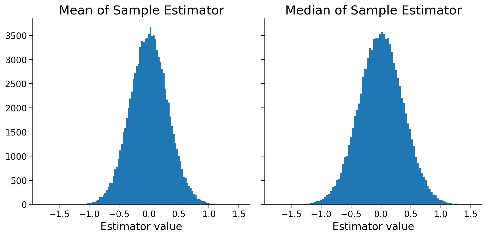
Is the median estimator biased or unbiased? Which estimator would you pick to use and why? Note that if things aren’t clear from the histogram, you are encouraged to compute the mean and variance of the two estimators (from the simulated values)

Answer

Text answer here

We can show that the variance of the sample mean estimator is \(Var(\hat{\mu}) = \frac{\sigma^2}{N}\) where N is the size of the sample. Thus, the variance decreasing with increasing sample size - this makes sense!

See here for a proof/explanation: https://online.stat.psu.edu/stat414/lesson/24/24.4.

Does the variance of the mean estimators from the simulations match this? Show this by computing the variance of these estimators and comparing to the analytical value.

Answer

# your code answer here

Text explanation here

B) Variance estimation

Remember that using the sample variance to estimate the population variance is biased? Let’s prove this to ourselves

n_samples = 100000
sample_size = 10

variance_estimators = np.zeros(n_samples,)
for i_sample in range(n_samples):
    sample = np.random.normal(size=(sample_size,))
    variance_estimators[i_sample] = np.var(sample)
fig, axes = plt.subplots(1, 1, figsize=(5, 5), sharey=True, sharex=True)
axes.hist(variance_estimators, 100);
axes.set(title='Variance of Sample Estimator', xlabel='Estimator value');

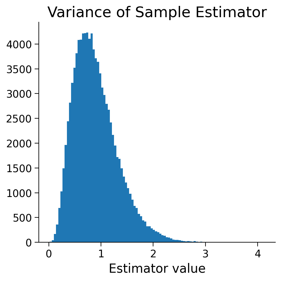
i) Prove to me that the variance of the sample is a biased estimator for the variance of the population. Note I’m not asking you the analytical proof (this is a bit long) but to show me based on the above simulation.

ii) Show that adjusting the estimator as described in the video (so the estimator is \(\hat{\sigma^2} = \frac{1}{N-1} \sum (X_i - \bar{X})^2)\) results in an unbiased estimator. (Do this by creating this new estimator - no need for analytical proof)

iii) Based on the simulations, is the variance of the original estimator (the variance of the sample, \(\hat{\sigma^2} = \frac{1}{N} \sum (X_i - \bar{X})^2)\)) or the adjusted estimator (\(\hat{\sigma^2} = \frac{1}{N-1} \sum (X_i - \bar{X})^2)\) higher? Which one has a higher mean squared error? Why do the answers to these two questions make sense together?

You will need to use code for all of these questions but also explain in text!

Answer

# your code here

Text explanation