Tutorial 2
Contents
![]()
Tutorial 2#
Linear Algebra II, Matrices
[insert your name]
Important reminders: Before starting, click “File -> Save a copy in Drive”. Produce a pdf for submission by “File -> Print” and then choose “Save to PDF”.
To complete this tutorial, you should have watched Videos 2.1 through 2.5.
Credits:
The videos you watched for this week were from 3Blue1Brown. Some elements of this problem set are from or inspired by https://openedx.seas.gwu.edu/courses/course-v1:GW+EngComp4+2019/about. In particular, we are using their plot_linear_transformation and plot_linear_transformations functions, and the demonstration of the additional transformation of a matrix inverse (end of Exercise 2)
# Imports
import numpy as np
import matplotlib.pyplot as plt
import matplotlib
import scipy.linalg

# Plotting parameters
matplotlib.rcParams.update({'font.size': 22})
Plotting functions#
# @title Plotting functions
import numpy
from numpy.linalg import inv, eig
from math import ceil
from matplotlib import pyplot, ticker, get_backend, rc
from mpl_toolkits.mplot3d import Axes3D
from itertools import cycle

def plot_range_3_by_2_matrix(matrix):

    fig = plt.figure()
    ax = fig.add_subplot(111, projection='3d')
    # Make data

    x = []
    y = []
    z = []
    for a1 in range(-10, 10, 1):
      for a2 in range(-10, 10, 1):
          vec = a1*matrix[:,0]+a2*matrix[:,1]
          x1, y1, z1 = vec
          x.append(x1)
          y.append(y1)
          z.append(z1)

    ax.scatter(np.array(x), np.array(y), np.array(z), color='b')

def plot_null_2_by_3_matrix(matrix):

    fig = plt.figure()
    ax = fig.add_subplot(111, projection='3d')
    # Make data

    basis = scipy.linalg.null_space(matrix)
    x = []
    y = []
    z = []
    for a1 in range(-10, 10, 1):
      for a2 in range(-10, 10, 1):

          vec = a1*basis[:,0]
          if basis.shape[1]==2:
            vec += a2*basis[:,1]
          x1, y1, z1 = vec
          x.append(x1)
          y.append(y1)
          z.append(z1)

    ax.scatter(np.array(x), np.array(y), np.array(z), color='b')


_int_backends = ['GTK3Agg', 'GTK3Cairo', 'MacOSX', 'nbAgg',
                 'Qt4Agg', 'Qt4Cairo', 'Qt5Agg', 'Qt5Cairo',
                 'TkAgg', 'TkCairo', 'WebAgg', 'WX', 'WXAgg', 'WXCairo']
_backend = get_backend()   # get current backend name

# shrink figsize and fontsize when using %matplotlib notebook
if _backend in _int_backends:
    fontsize = 4
    fig_scale = 0.75
else:
    fontsize = 5
    fig_scale = 1

grey = '#808080'
gold = '#cab18c'   # x-axis grid
lightblue = '#0096d6'  # y-axis grid
green = '#008367'  # x-axis basis vector
red = '#E31937'    # y-axis basis vector
darkblue = '#004065'

pink, yellow, orange, purple, brown = '#ef7b9d', '#fbd349', '#ffa500', '#a35cff', '#731d1d'

quiver_params = {'angles': 'xy',
                 'scale_units': 'xy',
                 'scale': 1,
                 'width': 0.012}

grid_params = {'linewidth': 0.5,
               'alpha': 0.8}

def set_rc(func):
    def wrapper(*args, **kwargs):
        rc('font', family='serif', size=fontsize)
        rc('figure', dpi=200)
        rc('axes', axisbelow=True, titlesize=5)
        rc('lines', linewidth=1)
        func(*args, **kwargs)
    return wrapper

@set_rc
def plot_vector(vectors, tails=None):
    ''' Draw 2d vectors based on the values of the vectors and the position of their tails.

    Parameters
    ----------
    vectors : list.
        List of 2-element array-like structures, each represents a 2d vector.

    tails : list, optional.
        List of 2-element array-like structures, each represents the coordinates of the tail
        of the corresponding vector in vectors. If None (default), all tails are set at the
        origin (0,0). If len(tails) is 1, all tails are set at the same position. Otherwise,
        vectors and tails must have the same length.

    Examples
    --------
    >>> v = [(1, 3), (3, 3), (4, 6)]
    >>> plot_vector(v)      # draw 3 vectors with their tails at origin
    >>> t = [numpy.array((2, 2))]
    >>> plot_vector(v, t)   # draw 3 vectors with their tails at (2,2)
    >>> t = [[3, 2], [-1, -2], [3, 5]]
    >>> plot_vector(v, t)   # draw 3 vectors with 3 different tails

    '''
    vectors = numpy.array(vectors)
    assert vectors.shape[1] == 2, "Each vector should have 2 elements."
    if tails is not None:
        tails = numpy.array(tails)
        assert tails.shape[1] == 2, "Each tail should have 2 elements."
    else:
        tails = numpy.zeros_like(vectors)

    # tile vectors or tails array if needed
    nvectors = vectors.shape[0]
    ntails = tails.shape[0]
    if nvectors == 1 and ntails > 1:
        vectors = numpy.tile(vectors, (ntails, 1))
    elif ntails == 1 and nvectors > 1:
        tails = numpy.tile(tails, (nvectors, 1))
    else:
        assert tails.shape == vectors.shape, "vectors and tail must have a same shape"

    # calculate xlimit & ylimit
    heads = tails + vectors
    limit = numpy.max(numpy.abs(numpy.hstack((tails, heads))))
    limit = numpy.ceil(limit * 1.2)   # add some margins

    figsize = numpy.array([2,2]) * fig_scale
    figure, axis = pyplot.subplots(figsize=figsize)
    axis.quiver(tails[:,0], tails[:,1], vectors[:,0], vectors[:,1], color=darkblue,
                  angles='xy', scale_units='xy', scale=1)
    axis.set_xlim([-limit, limit])
    axis.set_ylim([-limit, limit])
    axis.set_aspect('equal')

    # if xticks and yticks of grid do not match, choose the finer one
    xticks = axis.get_xticks()
    yticks = axis.get_yticks()
    dx = xticks[1] - xticks[0]
    dy = yticks[1] - yticks[0]
    base = max(int(min(dx, dy)), 1)   # grid interval is always an integer
    loc = ticker.MultipleLocator(base=base)
    axis.xaxis.set_major_locator(loc)
    axis.yaxis.set_major_locator(loc)
    axis.grid(True, **grid_params)

    # show x-y axis in the center, hide frames
    axis.spines['left'].set_position('center')
    axis.spines['bottom'].set_position('center')
    axis.spines['right'].set_color('none')
    axis.spines['top'].set_color('none')

@set_rc
def plot_transformation_helper(axis, matrix, *vectors, unit_vector=True, unit_circle=False, title=None):
    """ A helper function to plot the linear transformation defined by a 2x2 matrix.

    Parameters
    ----------
    axis : class matplotlib.axes.Axes.
        The axes to plot on.

    matrix : class numpy.ndarray.
        The 2x2 matrix to visualize.

    *vectors : class numpy.ndarray.
        The vector(s) to plot along with the linear transformation. Each array denotes a vector's
        coordinates before the transformation and must have a shape of (2,). Accept any number of vectors.

    unit_vector : bool, optional.
        Whether to plot unit vectors of the standard basis, default to True.

    unit_circle: bool, optional.
        Whether to plot unit circle, default to False.

    title: str, optional.
        Title of the plot.

    """
    assert matrix.shape == (2,2), "the input matrix must have a shape of (2,2)"
    grid_range = 20
    x = numpy.arange(-grid_range, grid_range+1)
    X_, Y_ = numpy.meshgrid(x,x)
    I = matrix[:,0]
    J = matrix[:,1]
    X = I[0]*X_ + J[0]*Y_
    Y = I[1]*X_ + J[1]*Y_
    origin = numpy.zeros(1)

    # draw grid lines
    for i in range(x.size):
        axis.plot(X[i,:], Y[i,:], c=gold, **grid_params)
        axis.plot(X[:,i], Y[:,i], c=lightblue, **grid_params)

    # draw (transformed) unit vectors
    if unit_vector:
        axis.quiver(origin, origin, [I[0]], [I[1]], color=green, **quiver_params)
        axis.quiver(origin, origin, [J[0]], [J[1]], color=red, **quiver_params)

    # draw optional vectors
    color_cycle = cycle([pink, darkblue, orange, purple, brown])
    if vectors:
        for vector in vectors:
            color = next(color_cycle)
            vector_ = matrix @ vector.reshape(-1,1)
            axis.quiver(origin, origin, [vector_[0]], [vector_[1]], color=color, **quiver_params)

    # draw optional unit circle
    if unit_circle:
        alpha =  numpy.linspace(0, 2*numpy.pi, 41)
        circle = numpy.vstack((numpy.cos(alpha), numpy.sin(alpha)))
        circle_trans = matrix @ circle
        axis.plot(circle_trans[0], circle_trans[1], color=red, lw=0.8)

    # hide frames, set xlimit & ylimit, set title
    limit = 4
    axis.spines['left'].set_position('center')
    axis.spines['bottom'].set_position('center')
    axis.spines['left'].set_linewidth(0.3)
    axis.spines['bottom'].set_linewidth(0.3)
    axis.spines['right'].set_color('none')
    axis.spines['top'].set_color('none')
    axis.set_xlim([-limit, limit])
    axis.set_ylim([-limit, limit])
    if title is not None:
        axis.set_title(title)

@set_rc
def plot_linear_transformation(matrix, *vectors, unit_vector=True, unit_circle=False):
    """ Plot the linear transformation defined by a 2x2 matrix using the helper
    function plot_transformation_helper(). It will create 2 subplots to visualize some
    vectors before and after the transformation.

    Parameters
    ----------
    matrix : class numpy.ndarray.
        The 2x2 matrix to visualize.

    *vectors : class numpy.ndarray.
        The vector(s) to plot along with the linear transformation. Each array denotes a vector's
        coordinates before the transformation and must have a shape of (2,). Accept any number of vectors.

    unit_vector : bool, optional.
        Whether to plot unit vectors of the standard basis, default to True.

    unit_circle: bool, optional.
        Whether to plot unit circle, default to False.

    """
    figsize = numpy.array([4,2]) * fig_scale
    figure, (axis1, axis2) = pyplot.subplots(1, 2, figsize=figsize)
    plot_transformation_helper(axis1, numpy.identity(2), *vectors, unit_vector=unit_vector, unit_circle=unit_circle, title='Before transformation')
    plot_transformation_helper(axis2, matrix, *vectors, unit_vector=unit_vector, unit_circle=unit_circle, title='After transformation')

@set_rc
def plot_linear_transformations(*matrices, unit_vector=True, unit_circle=False):
    """ Plot the linear transformation defined by a sequence of n 2x2 matrices using the helper
    function plot_transformation_helper(). It will create n+1 subplots to visualize some
    vectors before and after each transformation.

    Parameters
    ----------
    *matrices : class numpy.ndarray.
        The 2x2 matrices to visualize. Accept any number of matrices.

    unit_vector : bool, optional.
        Whether to plot unit vectors of the standard basis, default to True.

    unit_circle: bool, optional.
        Whether to plot unit circle, default to False.

    """
    nplots = len(matrices) + 1
    nx = 2
    ny = ceil(nplots/nx)
    figsize = numpy.array([2*nx, 2*ny]) * fig_scale
    figure, axes = pyplot.subplots(nx, ny, figsize=figsize)

    for i in range(nplots):  # fig_idx
        if i == 0:
            matrix_trans = numpy.identity(2)
            title = 'Before transformation'
        else:
            matrix_trans = matrices[i-1] @ matrix_trans
            if i == 1:
                title = 'After {} transformation'.format(i)
            else:
                title = 'After {} transformations'.format(i)
        plot_transformation_helper(axes[i//nx, i%nx], matrix_trans, unit_vector=unit_vector, unit_circle=unit_circle, title=title)
    # hide axes of the extra subplot (only when nplots is an odd number)
    if nx*ny > nplots:
        axes[-1,-1].axis('off')
Exercise 1: Don’t be a square#
In linear algebra, square matrices get a lot of the attention. We will often be dealing with m x n non-square matrices though, especially in neuroscience contexts! In this problem set, we’ll explore nonsquare matrices a bit more.
A) Rank & range if n < m#
i) If we have a 4 x 2 matrix A, what is the maximum possible rank of this matrix? (Hint: think about the columns of A)
ii) What does this mean for the range of the associated linear transformation? What is the maximum dimensionality subspace is can be?
iii) If we have an m x n matrix where n < m, can we ever reach every vector in \(R^m\)?
Your text answer
Play around below with inputting a 3 x 2 matrix and seeing the resulting range/column space in \(R^3\). In this plot, we’re taking all vectors with elements between -10 and 10 in \(R^2\) and plotting the transformed vector in \(R^3\).
First test a random matrix. Then create a matrix that results in a 1D line.
matrix = ...

plot_range_3_by_2_matrix(matrix)
---------------------------------------------------------------------------
TypeError                                 Traceback (most recent call last)
Cell In[3], line 3
      1 matrix = ...
----> 3 plot_range_3_by_2_matrix(matrix)

Cell In[2], line 20, in plot_range_3_by_2_matrix(matrix)
     18 for a1 in range(-10, 10, 1):
     19   for a2 in range(-10, 10, 1):
---> 20       vec = a1*matrix[:,0]+a2*matrix[:,1]
     21       x1, y1, z1 = vec
     22       x.append(x1)

TypeError: 'ellipsis' object is not subscriptable
B) Rank & range if m < n#
i) If we have a 2 x 4 matrix A, what is the maximum possible rank of this matrix?
ii) What is the minimum possible dimension of the null space for this matrix? (Hint: think about how space squishes)
Your text answer
Below, we’ll visualize the null space of a 2 x 3 matrix. Try out a random matrix and see what happens! Can you figure out how to make the null space 2D (Hint: take a look at Extra info: The Rank Theorem)?
matrix = ...
plot_null_2_by_3_matrix(matrix)
---------------------------------------------------------------------------
ValueError                                Traceback (most recent call last)
Cell In[4], line 2
      1 matrix = ...
----> 2 plot_null_2_by_3_matrix(matrix)

Cell In[2], line 34, in plot_null_2_by_3_matrix(matrix)
     31 ax = fig.add_subplot(111, projection='3d')
     32 # Make data
---> 34 basis = scipy.linalg.null_space(matrix)
     35 x = []
     36 y = []

File /opt/hostedtoolcache/Python/3.8.14/x64/lib/python3.8/site-packages/scipy/linalg/_decomp_svd.py:384, in null_space(A, rcond)
    331 def null_space(A, rcond=None):
    332     """
    333     Construct an orthonormal basis for the null space of A using SVD
    334
   (...)
    382
    383     """
--> 384     u, s, vh = svd(A, full_matrices=True)
    385     M, N = u.shape[0], vh.shape[1]
    386     if rcond is None:

File /opt/hostedtoolcache/Python/3.8.14/x64/lib/python3.8/site-packages/scipy/linalg/_decomp_svd.py:108, in svd(a, full_matrices, compute_uv, overwrite_a, check_finite, lapack_driver)
     13 def svd(a, full_matrices=True, compute_uv=True, overwrite_a=False,
     14         check_finite=True, lapack_driver='gesdd'):
     15     """
     16     Singular Value Decomposition.
     17
   (...)
    106
    107     """
--> 108     a1 = _asarray_validated(a, check_finite=check_finite)
    109     if len(a1.shape) != 2:
    110         raise ValueError('expected matrix')

File /opt/hostedtoolcache/Python/3.8.14/x64/lib/python3.8/site-packages/scipy/_lib/_util.py:290, in _asarray_validated(a, check_finite, sparse_ok, objects_ok, mask_ok, as_inexact)
    288 if not objects_ok:
    289     if a.dtype is np.dtype('O'):
--> 290         raise ValueError('object arrays are not supported')
    291 if as_inexact:
    292     if not np.issubdtype(a.dtype, np.inexact):

ValueError: object arrays are not supported

Extra info: Inverses of nonsquare matrices#
Nonsquare matrices do not have inverses. By definition, for matrix A, an inverse of A exists only if \(A^{-1}A = AA^{-1} = I_n\). If you have a nonsquare matrix A, you can never get the dimensions of \(A^{-1}\) to work.
Left and right inverses of nonsquare matrices do exist. If \(A\) is m x n and has rank equal to n, \(A\) has a left inverse \(B\) such that \(BA = I_n\), where \(B\) is n x m. If \(A\) has rank m, then is has a right inverse \(C\) such that \(AC = I_m\), where C is n x m.
Thinking through why the rank conditions in this definition are what they are is difficult but will help consolidate your knowledge if you want to try! Think about going from larger to smaller spaces vs smaller to larger spaces
Extra info: Determinants of nonsquare matrices#
Nonsquare matrices do not have determinants. Intuitively, determinants denote how much the associated linear transformation changes the area or volume of space covered. Because nonsquare matrices are transforming between dimensions, you cannot really compute the area changes since it changes dimensions (how do you compute the difference between an area and a volume).
Extra info: The Rank Theorem#
There is a theorem that says for an m x n matrix \(A\):
Basically the rank of a matrix plus the dimensionality of the null space must add up to the number of columns. We will see why this is true next week once we learn briefly how to solve matrix-vector equations by hand.
(Optional) Exercise 2: Changing basis#
In Video 1.3: Vector Spaces, we talked about changing basis (or changing coordinate systems). We looked at transforming a vector from a basis \(\beta = \{\bar{b}_1, \bar{b}_2\}\) where \(\bar{b}_1 = \begin{bmatrix} 1 \\ 1 \\ \end{bmatrix}\) and \(\bar{b}_2 = \begin{bmatrix} -1 \\ 1 \\ \end{bmatrix}\) to the standard basis. In particular, we had the \(\beta\) coordinates of vector \(\bar{a}\) (coordinates of a vector with respect to basis \(\beta\)) as \([\bar{a}]_{\beta} = \begin{bmatrix} 2 \\ 1 \\ \end{bmatrix}\). We computed the standard coordinates as:
A) Changing to the standard basis#
Now that we have learned about matrix multiplication, we can figure out how to change basis using it! We want to write a matrix P so that:
In other words, a matrix that transforms from the vector in coordinates relative to \(\beta\) to one with the coordinates relative to the standard basis. \(P_{\beta}\) is called the change-of-coordinates matrix from \(\beta\) to the standard basis.
What is \(P_{\beta}\) for the basis given above?
Hints: For the specific vector example,
You could find it by looking at the computation we did above and thinking how that could have been accomplished by a matrix multiplication or by thinking about what we learned this week: that matrices represent linear transformations and each column corresponds to where the corresponding basis vector ends up after the transformation.
Your math answer
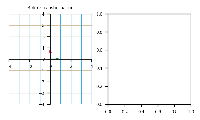
Fill in \(P_{\beta}\) below and plot the resulting linear transformation. This visualization highlights something essential: when we are in the basis \(\beta\) the \(\beta\) basis vectors seem like standard basis vectors. The Before transformation is when we are in “\(\beta-land\)” - it looks like when we are in standard basis vector land. It is only after we transform to standard coordinates, that we see the \(\beta\) vectors defined with respect to them (After transformation).
p_beta = ...

plot_linear_transformation(p_beta)
---------------------------------------------------------------------------
AttributeError                            Traceback (most recent call last)
Cell In[5], line 3
      1 p_beta = ...
----> 3 plot_linear_transformation(p_beta)

Cell In[2], line 88, in set_rc.<locals>.wrapper(*args, **kwargs)
     86 rc('axes', axisbelow=True, titlesize=5)
     87 rc('lines', linewidth=1)
---> 88 func(*args, **kwargs)

Cell In[2], line 263, in plot_linear_transformation(matrix, unit_vector, unit_circle, *vectors)
    261 figure, (axis1, axis2) = pyplot.subplots(1, 2, figsize=figsize)
    262 plot_transformation_helper(axis1, numpy.identity(2), *vectors, unit_vector=unit_vector, unit_circle=unit_circle, title='Before transformation')
--> 263 plot_transformation_helper(axis2, matrix, *vectors, unit_vector=unit_vector, unit_circle=unit_circle, title='After transformation')

Cell In[2], line 88, in set_rc.<locals>.wrapper(*args, **kwargs)
     86 rc('axes', axisbelow=True, titlesize=5)
     87 rc('lines', linewidth=1)
---> 88 func(*args, **kwargs)

Cell In[2], line 190, in plot_transformation_helper(axis, matrix, unit_vector, unit_circle, title, *vectors)
    164 @set_rc
    165 def plot_transformation_helper(axis, matrix, *vectors, unit_vector=True, unit_circle=False, title=None):
    166     """ A helper function to plot the linear transformation defined by a 2x2 matrix.
    167
    168     Parameters
   (...)
    188
    189     """
--> 190     assert matrix.shape == (2,2), "the input matrix must have a shape of (2,2)"
    191     grid_range = 20
    192     x = numpy.arange(-grid_range, grid_range+1)

AttributeError: 'ellipsis' object has no attribute 'shape'
B) Changing from the standard basis#
Luckily for us, the matrix \(P_{\beta}\) is always invertible. We know this from the Invertible Matrix Theorem presented in Part 1 because the columns of \(P_{\beta}\) span \(R^n\) (since they are a basis for \(R^n\)). So we can compute the coordinates of a vector with respect to \(\beta\) as:
We will compute \(P^{-1}_{\beta}\) using code and find the \(\beta\) coordinates of \(\bar{x} = \begin{bmatrix} 4 \\ 2\\ \end{bmatrix}\)
p_beta_inverse = ...

beta_coordinates = ...

print(beta_coordinates)
Ellipsis
C) Changing basis criterion#
Not every matrix-vector multiplication can be considered a change of basis. What has to be true of the matrix for it to be a change of basis?
Your text answer
Extra info: Changing between two non-standard bases#
We can also change from basis \(\beta\) to another basis \(C\) without first moving to the standard basis. We will not get into this here due to time constraints but you should have all the tools to understand the explanation here if you wish: https://math.berkeley.edu/~arash/54/notes/04_07.pdf