Tutorial 1#

Probability & Statistics II: Intro to Statistics

[insert your name]

Important reminders: Before starting, click “File -> Save a copy in Drive”. Produce a pdf for submission by “File -> Print” and then choose “Save to PDF”.

To complete this tutorial, you should have watched Videos 7.1 - 7.5

Imports

# @markdown Imports

# Imports

import numpy as np
import matplotlib.pyplot as plt
import ipywidgets as widgets  # interactive display
import math

Plotting functions

# @markdown Plotting functions
import numpy
from numpy.linalg import inv, eig
from math import ceil
from matplotlib import pyplot, ticker, get_backend, rc
from mpl_toolkits.mplot3d import Axes3D
from itertools import cycle


%config InlineBackend.figure_format = 'retina'
plt.style.use("https://raw.githubusercontent.com/NeuromatchAcademy/course-content/master/nma.mplstyle")

Exercise 1: Clarifying Correlation#

There are a lot of misunderstandings over what information correlation coefficients capture so let’s make completely sure we understand this descriptive statistics.

A) Simulate data#

We are looking at two variables, x and y, and the relationship between them. We will simulate x from a normal distribution with mean 5 and standard deviation 1.
$$ x = N(5 | 1)$$

This notation $N(\mu | \sigma)$ denotes a normal (Gaussian) distribution with mean $\mu$ and standard deviation $\sigma$.

We will model y as:

\[ y = c (x + N (0, \sigma)) + N(0, \sigma)\]

c here is a constant the determines the slope of the relationship and $\sigma$ denotes the size of the noise added to get y (added to x before multiplication with the slope and again afterwards).

Complete the function below to simulate x and y for a given slope and noise standard deviation and compute the correlation coefficient between them. You can use np.random.normal and np.corrcoef which gives the Pearson correlation coefficient (the commonly used metric), which measures the linear correlation between two variables as:

\[ r = \frac{\sum (x_i - \bar{x})(y_i - \bar{y})}{\sqrt{\sum(x_i - \bar{x})^2\sum(y_i - \bar{y})^2}} \]

Hint: a normal distribution $N(\mu | \sigma)$ is equivalent to $\mu + \sigma N(0|1)$.

def simulate_data(slope, noise_sd, n_data_points = 300):

  # Simulate x
  x = ...

  # Simulate y
  y = ...
  
  # Get correlation coefficient
  corr_coef = ...

  return x, y, corr_coef

A) Correlation vs noise#

We will first assume the slope is equal to 2 and vary the standard deviation of the noise.

Execute this cell to plot simulated data

# @markdown Execute this cell to plot simulated data
slope = 2
noise_sds = np.arange(0, 10, 2)

fig, axes = plt.subplots(1, 5, figsize=(20, 4)) #, sharey=True, sharex=True)
r, c = (0, 0)

corr_coefs = np.zeros((noise_sds.shape[0],))
for i_noise, noise_sd in enumerate(noise_sds):
  x, y, corr_coef = simulate_data(slope, noise_sd)
  corr_coefs[i_noise] = corr_coef
  axes[i_noise].plot(x, y, '.')
  axes[i_noise].set_aspect('auto')
  c+=1
  if c > 4:
    r += 1
    c = 0
  axes[i_noise].set(title ='Noise sd = '+str(noise_sd), xlabel = 'x')

---------------------------------------------------------------------------
TypeError                                 Traceback (most recent call last)
Cell In[4], line 11
      9 for i_noise, noise_sd in enumerate(noise_sds):
     10   x, y, corr_coef = simulate_data(slope, noise_sd)
---> 11   corr_coefs[i_noise] = corr_coef
     12   axes[i_noise].plot(x, y, '.')
     13   axes[i_noise].set_aspect('auto')

TypeError: float() argument must be a string or a number, not 'ellipsis'

Before executing next cell Guess the correlation coefficient for each of these 5 plots and draw a plot of those correlation coefficients vs the noise (so y axis is correlation coefficient and x axis is noise sd). Note that this graph won’t be graded on accuracy but you will be expected to submit it.

Answer#

Put your graph here

Now we will look at the actual graph below.

AFTER PREVIOUS STEP: Execute this cell to plot correlation coefficients vs noise sd

# @markdown AFTER PREVIOUS STEP: Execute this cell to plot correlation coefficients vs noise sd

fig, ax = plt.subplots(figsize=(5, 5))
ax.plot(noise_sds, corr_coefs, 'o-', c='#70E0BD', lw=3)

ax.set(title='Correlation coefficient vs noise', xlabel='Noise sd', ylabel='Corr coeff');

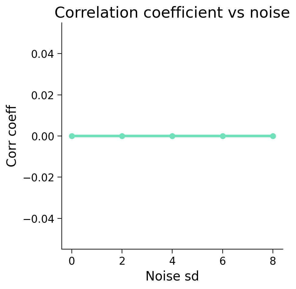
Does this graph look different than the one you had predicted? If so, how?

Answer#

Text answer here

B) Correlation vs slope of relationship#

Now we will assume a constant standard deviation of 1 and vary the slope.

Execute this cell to plot simulated data

# @markdown Execute this cell to plot simulated data
noise_sd = 1
slopes = np.arange(-8, 9, 2)

fig, axes = plt.subplots(1, len(slopes), figsize=(20, 4), sharey=True, sharex=True)
r, c = (0, 0)

corr_coefs = np.zeros((slopes.shape[0],))
for i_slope, slope in enumerate(slopes):
  x, y, corr_coef = simulate_data(slope, noise_sd)
  corr_coefs[i_slope] = corr_coef
  axes[i_slope].plot(x, y, '.')
  axes[i_slope].set_aspect('auto')
  c+=1
  if c > 4:
    r += 1
    c = 0
  axes[i_slope].set(title ='Slope = '+str(slope), xlabel = 'x')

---------------------------------------------------------------------------
TypeError                                 Traceback (most recent call last)
Cell In[6], line 11
      9 for i_slope, slope in enumerate(slopes):
     10   x, y, corr_coef = simulate_data(slope, noise_sd)
---> 11   corr_coefs[i_slope] = corr_coef
     12   axes[i_slope].plot(x, y, '.')
     13   axes[i_slope].set_aspect('auto')

TypeError: float() argument must be a string or a number, not 'ellipsis'

Before executing next cell Guess the correlation coefficient for each of these 9 plots and draw a plot of those correlation coefficients vs the slope (so y axis is correlation coefficient and x axis is slope). Note that this graph won’t be graded on accuracy but you will be expected to submit it.

Answer#

Put your graph here

AFTER PREVIOUS STEP: Execute this cell to plot correlation coefficients vs slope

# @markdown AFTER PREVIOUS STEP: Execute this cell to plot correlation coefficients vs slope

fig, ax = plt.subplots(figsize=(5, 5))
ax.plot(slopes, corr_coefs, 'o-', c='#70E0BD', lw=3)

ax.set(title='Correlation coefficient vs slope', xlabel='Slope', ylabel='Corr coeff');

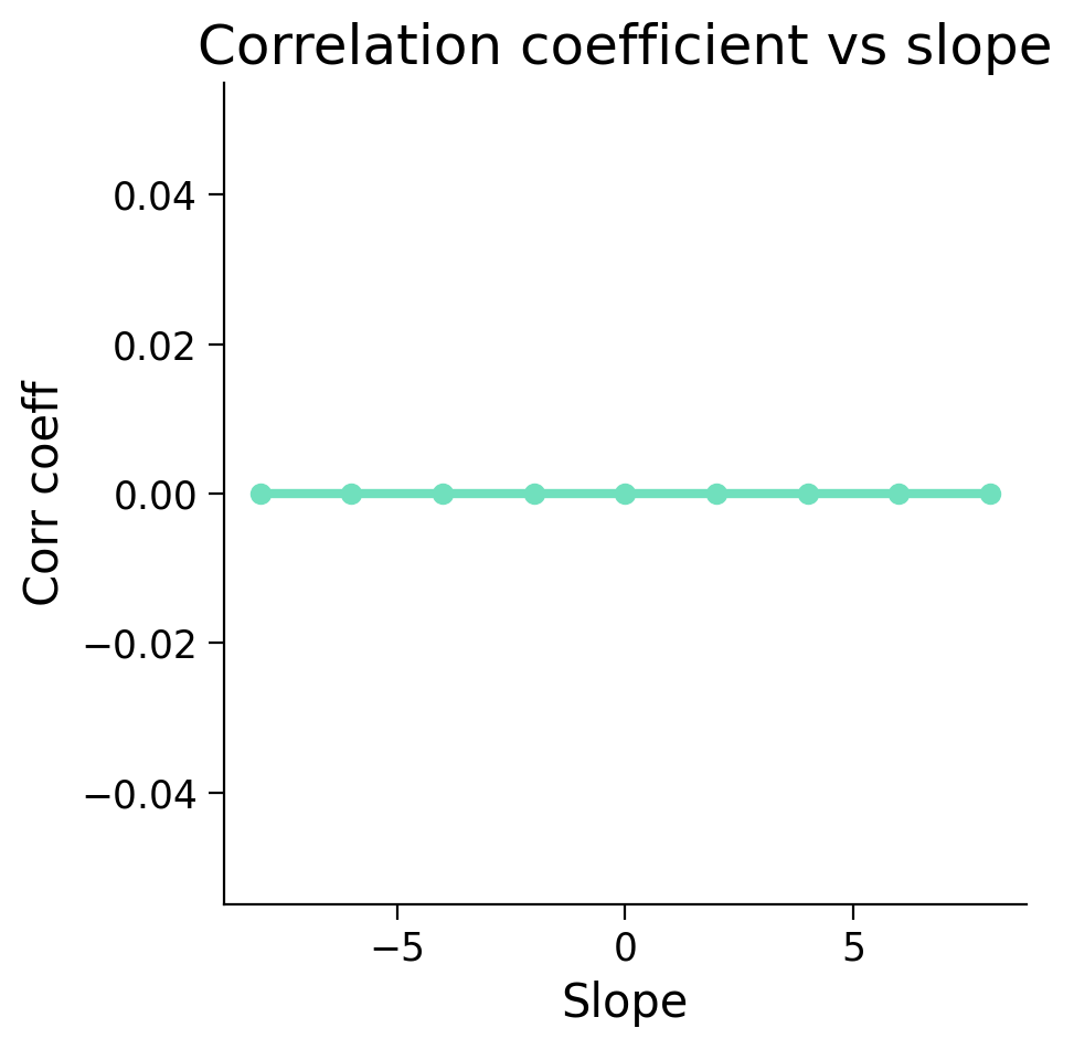
Does this graph look different than the one you had predicted? If so, how?

Answer#

Text answer here

C) Variable relationships with zero correlation#

Draw a scatter plot of x and y where there is a clear relationship between them but they would have a correlation coefficient of 0. You can draw this by hand or make the data points and plot in matplotlib (the added benefit being you can check the correlation is almost 0).

Why would your x/ys have a correlation coefficient of 0?

Answer#

Put your graph here

Answer#

Text answer here

Extra info

Another common misunderstanding is between correlation and causation. Even if x and y have a correlation of 1, we cannot say that one causes the other. There could be other additional factors that lead to x and y being highly correlated without being causal.

Exercise 2: Decoding head direction#

In this exercise we will again use the neural responses to head direction we outlined in Week 6 Tutorial 1.

Let’s say we just the neural response (spike count) and want to guess the head direction that the mouse is at. This is called decoding. In decoding generally, we are trying to reconstruct some stimulus or behavior from the neural responses.

A) Maximizing likelihood estimator#

If we know the probability of the spike count given the head direction, one option is to guess the the head direction that maximizes that probability. We do know this probability mapping - it’s our Poisson distribution from Exercise 1. In particular, $P(S = k | H = \theta)$ is our likelihood: the probability of spike count k given the head direction at that point in time, or $\theta$ .

$$ P(S = k | H = \theta) = \frac{\lambda ^k e^{-\lambda}}{k!} $$ where $\lambda = \frac{1}{20}\theta$.

If our spike count is 15, what is your guess of $\theta$ given this spike count?

Let’s solve this using a brute force coding method: loop over possible $\theta s$, compute $P(S = k | H = \theta)$ for each, and then find which $\theta$ maximizes that quantity.

You may want to use np.math.factorial

thetas = np.arange(0, 360, 1)

k = 15
likelihoods = np.zeros((len(thetas),))
for i, theta in enumerate(thetas):
  ...

# Get theta that maximizes the likelihood
theta_max_likelihood = ...
print(theta_max_likelihood)

Ellipsis

fig, ax = plt.subplots(1, 1)
ax.plot(thetas, likelihoods, 'k')
ax.set(xlabel='Theta', ylabel='P(S= 15 | H=theta)');

Answer#

Answer here

B) Incorporating priors#

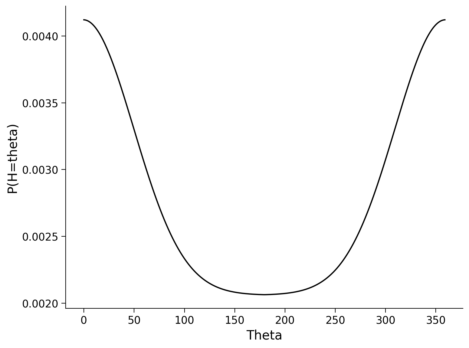
We notice however that the mouse spends much more time in certain head directions than others. In particular, the mouse spends a lot of time facing forward, which is at $\theta=0$. We get the probability that the mouse is at each $\theta$ by computing the fraction of time she spends at that head direction. I give this to you below (prior_prob) - see plot below.

Execute this cell to get and visualize prior_prob

# @markdown Execute this cell to get and visualize prior_prob 

import scipy.signal

gauss = scipy.signal.gaussian(360, 50, sym=True)+1
gauss /= np.sum(gauss)
prior_prob = np.concatenate((gauss[int(360/2):], gauss[:int(360/2)]))

fig, ax = plt.subplots(1, 1)
ax.plot(thetas, prior_prob, 'k')
ax.set(xlabel='Theta', ylabel='P(H=theta)');

We think we can get a more accurate guess of head direction given the spike count of 15 by incorporating the additional information of how likely the mouse is to be at each head direction (our prior on head direction).

Luckily, we have a nice way to do this using Bayes Theorem! In particular,

\[ P(H = \theta | S = k) = \frac{P(S=k|H=\theta)P(H=\theta)}{P(S=k)}\]

We now want to guess the head direction that lead to a spike count of 15 by maximing $P(H = \theta | S = k)$, our posterior, instead of $P(S = k | H = \theta)$, our likelihood. We can drop the denominator $P(S=k)$ because this is constant across head directions so won’t affect our guess.

\[ P(H = \theta | S = k) \propto P(S=k|H=\theta)P(H=\theta)\]

What $\theta$ would we guess the mouse is at if we maximize $P(H = \theta | S = k)$?

We can again use the brute force method.

k = 15
posterior_probs = np.zeros((len(thetas),))
for i, theta in enumerate(thetas):
  ...


# Get theta that maximizes the posterior probability
theta_max_posterior = ...
print(theta_max_posterior)

Ellipsis

fig, ax = plt.subplots(1, 1)
ax.plot(thetas, posterior_probs, 'k')
ax.set(xlabel='Theta', ylabel='Proportional to P(H=theta | S= 15)');

Answer#

Answer here

C) Comparison#

Compare the guess of $\theta$ in A vs B. Why does it make sense that the difference is what it is? Aka, how and why did the prior over head direction effect the guess the way it did?

Answer#

Answer here

Exercise 3: MLE Derivation for Binomial Distribution#

We can model a single coin flip using the Bernoulli distribution: $$ P( k | p ) = p^k (1-p)^{1-k} $$

where p is the probability of the coin coming up heads and k indicates heads vs tails (k = 1 is heads, k = 0 is tails).

We can model a series of coin flips using the binomial distribution; we obtain a binomial distribution by summing up n independent Bernoulli random variables Ber(p), each of which has probability p of coming up heads. A binomial distribution is:

\[ p( k | n, p) = \binom{n}{k}p^k (1-p)^{n-k} \]

where $\binom{n}{k}$ is a binomial coefficient (n choose k) equal to $\frac{n!}{k!(n-k)!}$. This counts the number of different ways you can get k heads from n flipped coins and is essentially there to make the distribution sum to 1. Let’s derive the equation for the maximum likelihood estimator for p in a binomial distribution.

Show your work!

Answer#

Answer here

Major hint

# @markdown Major hint

# Take the derivative of the log likelihood and
# set equal to 0

Mathematical Tools for Neuroscientists

Tutorial 1

Contents

Tutorial 1#

Exercise 1: Clarifying Correlation#

A) Simulate data#

A) Correlation vs noise#

Answer#

Answer#

B) Correlation vs slope of relationship#

Answer#

Answer#

C) Variable relationships with zero correlation#

Answer#

Answer#

Exercise 2: Decoding head direction#

A) Maximizing likelihood estimator#

Answer#

B) Incorporating priors#

Answer#

C) Comparison#

Answer#

Exercise 3: MLE Derivation for Binomial Distribution#

Answer#