Tutorial 1
Contents
![]()
Tutorial 1#
Machine Learning I: Linear & Logistic Regression
[insert your name]
Important reminders: Before starting, click “File -> Save a copy in Drive”. Produce a pdf for submission by “File -> Print” and then choose “Save to PDF”.
To complete this tutorial, you should have watched Video 9.1 - 9.3.
Imports
# @markdown Imports

# Imports
import numpy as np
import matplotlib.pyplot as plt
import ipywidgets as widgets  # interactive display
import math
import scipy.stats
from ipywidgets import *
Plotting functions
# @markdown Plotting functions
import numpy
from numpy.linalg import inv, eig
from math import ceil
from matplotlib import pyplot, ticker, get_backend, rc
from mpl_toolkits.mplot3d import Axes3D
from itertools import cycle


%config InlineBackend.figure_format = 'retina'
plt.style.use("https://raw.githubusercontent.com/NeuromatchAcademy/course-content/master/nma.mplstyle")

def plot_line_diff_residuals(x, y, slope):
  """ Plot observed vs predicted data

  Args:
      x (ndarray): observed x values
      y (ndarray): observed y values
      theta_hat (scalar): estimate for slope of line
  """

  x_range = np.arange(-10, 10, .1)
  fig, ax = plt.subplots()
  ax.scatter(x, y)  # our data scatter plot
  ax.plot(x_range, slope*x_range, color='k')

  # plot green lines
  y_hat = slope * x
  ymin = np.minimum(y, y_hat)
  ymax = np.maximum(y, y_hat)
  ax.vlines(x, ymin, ymax, 'g', alpha=0.5)

  # plot red lines
  data = np.concatenate(((x[:, None], y[:, None])), axis=1)
  theta = np.arctan(slope)

  w = np.asarray([np.cos(theta), np.sin(theta)])[None, :];

  z = data @ w.T @ w;
  dists = np.zeros((x.shape[0]))
  for i in range(x.shape[0]):
    ax.plot([data[i,0], z[i,0]], [data[i,1], z[i,1]], 'r')
    dists[i] = np.sqrt((z[i, 0] - data[i, 0])**2 + (z[i, 1] - data[i, 1])**2)

  ax.set(xlim=[-7, 7], ylim = [-7, 7])

  # Compute sum of squared lengths of residuals
  A = np.mean((y_hat-y)**2)

  B = np.mean(dists**2)
  ax.set_aspect('equal')
  ax.set(
      title=fr"$\hat{{\theta}}$ = {slope:0.2f}, A = {A:.3f}, B = {B:.3f}",
      xlabel='x',
      ylabel='y'
  )
Exercise 1: PCA vs Linear Regression#
This demo is inspired by (but quite changed) from NMA W1D3 T1.
We are going to explore the difference between the first PCA component and the linear regression line when both x and y are 1D. Play with the interactive demo and then answer the questions below. We are simulating data (the blue dots): both x and y are mean centered. You can then manipulate the slope of the plotted line and see how it affects the green lines vs the red lines.
In the title, A is the summed squared length of the green lines. B is the summed squared length of the red lines.
Execute this cell to enable the demo
#@markdown Execute this cell to enable the demo

# Simulate some data
np.random.seed(121)

# Let's set some parameters
theta = 1.2
n_samples = 30

# Draw x and then calculate y
x = 10 * np.random.rand(n_samples)-5 # sample from a uniform distribution over [0,10)
noise = np.random.randn(n_samples)  # sample from a standard normal distribution
y = theta * x + noise

x = x - np.mean(x)
y = y - np.mean(y)

@widgets.interact(slope=widgets.FloatSlider(1.1, min=1.2, max=1.45, step=0.01 ))
def plot_data_estimate(slope):

  plot_line_diff_residuals(x, y, slope)
i) What slope gives the linear regression line (predicting y from x)?
ii) Why?
iii) What slope gives the first principal component of the data?
iv) Why?
Answer#
i)
ii)
iii)
iV)
Exercise 2: Least squares solution for multiple linear regression#
This problem was adapted from (and uses code from) NMA W1D3 T4.
Let’s assume we are trying to decode the mouse running speed from the firing rates of two neurons. We are assuming a linear model so:
where y is the running speed and \(x_1\) and \(x_2\) are the firing rates of the two neurons respectively.
Remember that if we pose this problem in matrix form:
the vector \(\theta\) that miminimizes the mean squared error between the predicted and true running speeds is:
Here y is a vector of running speeds where the length is the number of data points. X is the design matrix involving the inputs and \(\bar{\theta}\) is a vector of weights on the components of the design matrix.
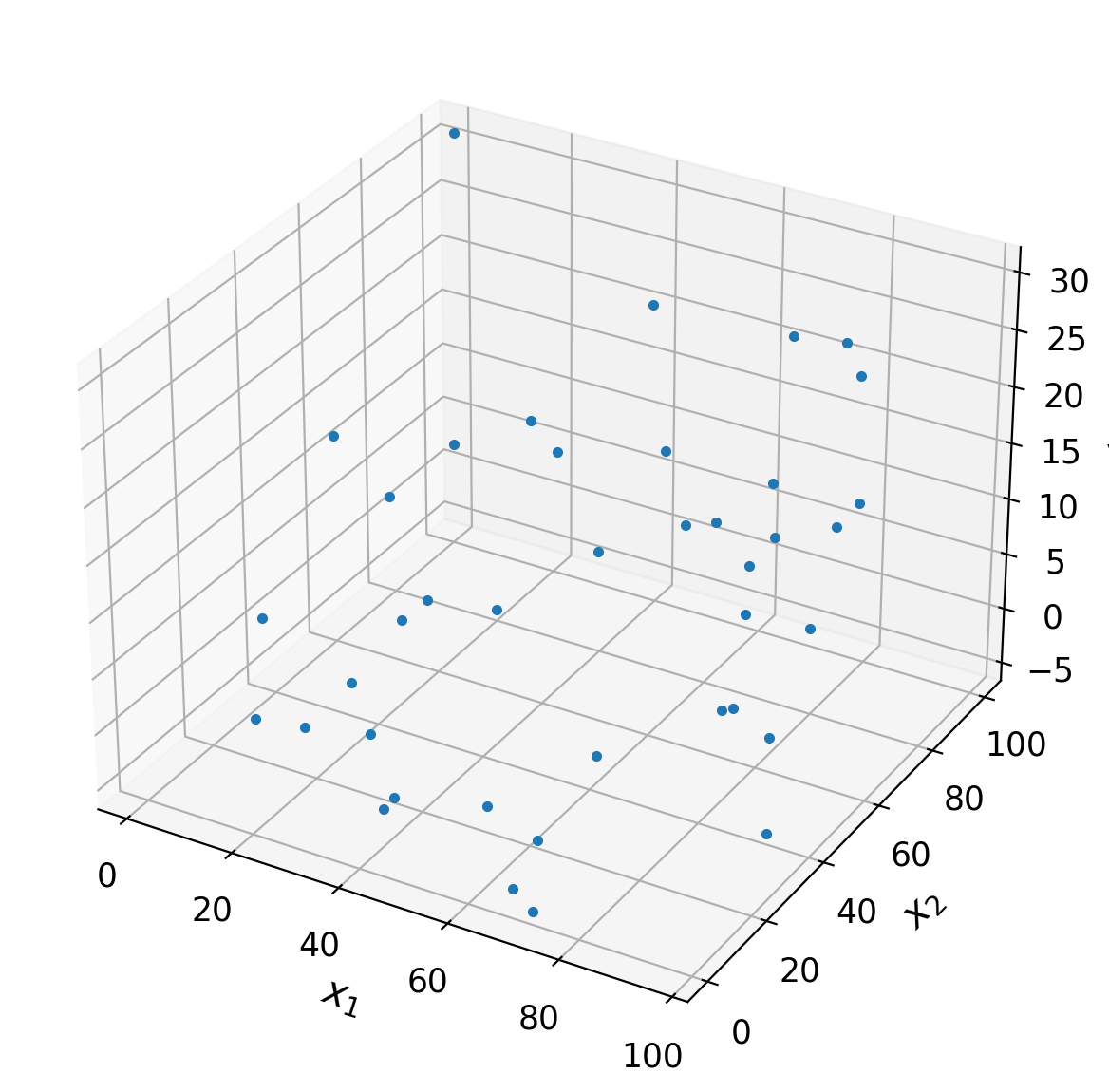
Execute the cell below to generate the data we will fit our linear regression model to. The variables are called y, x1, and x2.
Execute this cell to generate data
# @markdown Execute this cell to generate data

# Set random seed for reproducibility
np.random.seed(1234)

# Set parameters
theta = [1, -.1, .3]
n_samples = 40

# Draw x and calculate y

x1 = np.random.uniform(0, 100, (n_samples, 1))
x2 = np.random.uniform(0, 100, (n_samples, 1))
noise = 5*np.random.randn(n_samples, 1)
y = theta[0] + theta[1]*x1 + theta[2]*x2 + noise


ax = plt.subplot(projection='3d')
ax.plot(x1[:, 0], x2[:, 0], y[:, 0], '.')

ax.set(
    xlabel='$x_1$',
    ylabel='$x_2$',
    zlabel='y'
)
plt.tight_layout()
A) Create design matrix#
Create the design matrix \(X\) so that the matrix form matches the first equation above.
Answer#
Code below
# your code here
X = ...
B) Implement least squares solution#
Complete the function below to compute the least squares solution to estimate \(\bar{\theta}\).
Answer#
Code below
def ordinary_least_squares(X, y):
  """Ordinary least squares estimator for linear regression.

  Args:
    x (ndarray): design matrix of shape (n_samples, n_regressors)
    y (ndarray): vector of measurements of shape (n_samples)

  Returns:
    ndarray: estimated parameter values of shape (n_regressors)
  """

  # Compute theta_hat using OLS
  theta_hat = ...

  return theta_hat


theta_hat = ordinary_least_squares(X, y)
print(theta_hat)
Ellipsis
C) Compute MSE#
Below, compute the mean square error between your predictions using the linear regression model and the true values of y.
Remember that your predictions are: $\(\hat{y} = X\hat{\theta} \)$
Answer#
Code below
y_hat = ...

MSE = ...
print(MSE)
Ellipsis
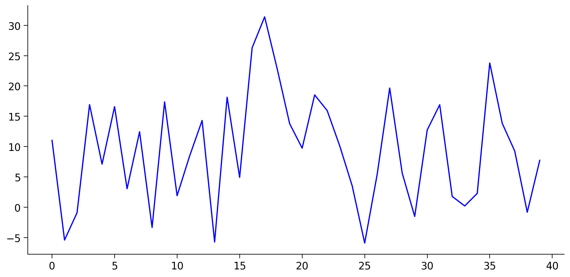
D) Thinking about what the model tells us#
Execute this cell to visualize predictions
# @markdown Execute this cell to visualize predictions

fig, ax = plt.subplots(figsize=(10, 5))
ax.plot(y, 'b', label = 'True')
ax.plot(y_hat, 'r', label = 'Predicted')
ax.legend()
ax.set(xlabel='Data points', ylabel='Running speed');
---------------------------------------------------------------------------
TypeError                                 Traceback (most recent call last)
Cell In[8], line 5
      3 fig, ax = plt.subplots(figsize=(10, 5))
      4 ax.plot(y, 'b', label = 'True')
----> 5 ax.plot(y_hat, 'r', label = 'Predicted')
      6 ax.legend()
      7 ax.set(xlabel='Data points', ylabel='Running speed');

File /opt/hostedtoolcache/Python/3.8.14/x64/lib/python3.8/site-packages/matplotlib/axes/_axes.py:1664, in Axes.plot(self, scalex, scaley, data, *args, **kwargs)
   1662 lines = [*self._get_lines(*args, data=data, **kwargs)]
   1663 for line in lines:
-> 1664     self.add_line(line)
   1665 if scalex:
   1666     self._request_autoscale_view("x")

File /opt/hostedtoolcache/Python/3.8.14/x64/lib/python3.8/site-packages/matplotlib/axes/_base.py:2340, in _AxesBase.add_line(self, line)
   2337 if line.get_clip_path() is None:
   2338     line.set_clip_path(self.patch)
-> 2340 self._update_line_limits(line)
   2341 if not line.get_label():
   2342     line.set_label(f'_child{len(self._children)}')

File /opt/hostedtoolcache/Python/3.8.14/x64/lib/python3.8/site-packages/matplotlib/axes/_base.py:2363, in _AxesBase._update_line_limits(self, line)
   2359 def _update_line_limits(self, line):
   2360     """
   2361     Figures out the data limit of the given line, updating self.dataLim.
   2362     """
-> 2363     path = line.get_path()
   2364     if path.vertices.size == 0:
   2365         return

File /opt/hostedtoolcache/Python/3.8.14/x64/lib/python3.8/site-packages/matplotlib/lines.py:1031, in Line2D.get_path(self)
   1029 """Return the `~matplotlib.path.Path` associated with this line."""
   1030 if self._invalidy or self._invalidx:
-> 1031     self.recache()
   1032 return self._path

File /opt/hostedtoolcache/Python/3.8.14/x64/lib/python3.8/site-packages/matplotlib/lines.py:664, in Line2D.recache(self, always)
    662 if always or self._invalidy:
    663     yconv = self.convert_yunits(self._yorig)
--> 664     y = _to_unmasked_float_array(yconv).ravel()
    665 else:
    666     y = self._y

File /opt/hostedtoolcache/Python/3.8.14/x64/lib/python3.8/site-packages/matplotlib/cbook/__init__.py:1369, in _to_unmasked_float_array(x)
   1367     return np.ma.asarray(x, float).filled(np.nan)
   1368 else:
-> 1369     return np.asarray(x, float)

TypeError: float() argument must be a string or a number, not 'ellipsis'
Execute to see the fitted plane
# @markdown Execute to see the fitted plane
theta_hat = ordinary_least_squares(X, y)
xx, yy = np.mgrid[0:100:50j, 0:100:50j]
y_hat_grid = np.array([xx.flatten(), yy.flatten()]).T @ theta_hat[1:]
y_hat_grid = y_hat_grid.reshape((50, 50))

ax = plt.subplot(projection='3d')
ax.plot(X[:, 1], X[:, 2], y[:, 0], '.')
ax.plot_surface(xx, yy, y_hat_grid, linewidth=0, alpha=0.5, color='C1',
                cmap=plt.get_cmap('coolwarm'))

ax.set(
    xlabel='$x_1$',
    ylabel='$x_2$',
    zlabel='y'
)
plt.tight_layout()
---------------------------------------------------------------------------
TypeError                                 Traceback (most recent call last)
Cell In[9], line 4
      2 theta_hat = ordinary_least_squares(X, y)
      3 xx, yy = np.mgrid[0:100:50j, 0:100:50j]
----> 4 y_hat_grid = np.array([xx.flatten(), yy.flatten()]).T @ theta_hat[1:]
      5 y_hat_grid = y_hat_grid.reshape((50, 50))
      7 ax = plt.subplot(projection='3d')

TypeError: 'ellipsis' object is not subscriptable
Based on these plots and \(\hat{\theta}\):
i) Do you think neurons 1 and 2 contain information about running speed in their responses?
ii) If we were going to interpret the weights (which we should be very careful about!!!), what effect would you say neuron 1 firing a lot has on the running speed?
iii) What effect does neuron 2 firing a lot have on the running speed?
Note we cannot say anything causal here - we cannot say if the firing of the neurons is changing the running speed, if the running speed is affecting the neurons, or if there is some third variable that affects both.
Answer#
i)
ii)
iii)
Exercise 3 (Optional): MLE for linear regression#
Prove that the MLE for the linear model assuming Gaussian noise is the same as the least squares solution. Do this either for 1D inputs or multidimensional inputs (more advanced)
Answer#
Answer here