Tutorial 2#

Machine Learning II, Model Selection

[insert your name]

Important reminders: Before starting, click “File -> Save a copy in Drive”. Produce a pdf for submission by “File -> Print” and then choose “Save to PDF”.

To complete this tutorial, you should have watched Video 10.1, 10.2, and 10.3

This tutorial is inspired by and uses text/code from NMA W1D4

Imports

# @markdown Imports

# Imports
import numpy as np
import matplotlib.pyplot as plt
import ipywidgets as widgets  # interactive display
import math

import matplotlib as mpl
from sklearn.linear_model import LinearRegression, Lasso, Ridge

---------------------------------------------------------------------------
ModuleNotFoundError                       Traceback (most recent call last)
Cell In[1], line 10
      7 import math
      9 import matplotlib as mpl
---> 10 from sklearn.linear_model import LinearRegression, Lasso, Ridge

ModuleNotFoundError: No module named 'sklearn'

Plotting functions

# @markdown Plotting functions
import warnings
warnings.simplefilter(action='ignore', category=FutureWarning)

import numpy
from numpy.linalg import inv, eig
from math import ceil
from matplotlib import pyplot, ticker, get_backend, rc
from mpl_toolkits.mplot3d import Axes3D
from itertools import cycle


%config InlineBackend.figure_format = 'retina'
plt.style.use("https://raw.githubusercontent.com/NeuromatchAcademy/course-content/master/nma.mplstyle")

def plot_weights(models, sharey=True):
  """Draw a stem plot of weights for each model in models dict."""
  n = len(models)
  f = plt.figure(figsize=(10, 2.5 * n))
  axs = f.subplots(n, sharex=True, sharey=sharey)
  axs = np.atleast_1d(axs)

  for ax, (title, model) in zip(axs, models.items()):

    ax.margins(x=.02)
    stem = ax.stem(model.coef_.squeeze(), use_line_collection=True)
    stem[0].set_marker(".")
    stem[0].set_color(".2")
    stem[1].set_linewidths(.5)
    stem[1].set_color(".2")
    stem[2].set_visible(False)
    ax.axhline(0, color="C3", lw=3)
    ax.set(ylabel="Weight", title=title)
  ax.set(xlabel="Neuron (a.k.a. feature)")
  f.tight_layout()

def plot_model_quality(run_train, preds_train, run_test, preds_test, r2_train, r2_test):
  fig, axes = plt.subplots(1, 3, figsize=(15, 5))

  axes[0].plot(run_train[:500],'k', label = 'True running speed')
  axes[0].plot(preds_train[:500],'g',alpha=.7, label = 'Predicted running speed')

  axes[0].legend()

  axes[1].plot(run_test[:500],'k')
  axes[1].plot(preds_test[:500],'g',alpha=.7)

  axes[2].bar([0, 1], [r2_train, r2_test])

  axes[0].set(title='Training data', xlabel='Time (bins)', ylabel='Running speed')
  axes[1].set(title='Validation  data', xlabel='Time (bins)', ylabel='Running speed')
  axes[2].set(title='Prediction Quality', ylabel='R2', xticks = [0, 1], xticklabels = ['Training data', 'Validation data']);


def plot_regularized_train_and_val(alphas, reg_train_r2s, reg_validation_r2s, train_r2, validation_r2, regression_type):
    fig, axes = plt.subplots(1, 2, figsize=(10, 5))

    axes[0].plot([0, len(alphas)], [train_r2, train_r2], 'g', label= 'No reg')
    axes[0].plot(reg_train_r2s, '-ob', label = regression_type)
    axes[0].set(title='Training data', ylabel='R2', xlabel='alpha', xticks = np.arange(0, len(alphas)), xticklabels = alphas)

    axes[0].legend()

    axes[1].plot([0, len(alphas)], [validation_r2, validation_r2], 'g')
    axes[1].plot(reg_validation_r2s, '-ob')
    axes[1].set(title='Validation data', ylabel='R2', xlabel='alpha', xticks = np.arange(0, len(alphas)), xticklabels= alphas);

Data retrieval

#@markdown Data retrieval
import os, requests

fname = "stringer_spontaneous.npy"
url = "https://osf.io/dpqaj/download"

if not os.path.isfile(fname):
  try:
    r = requests.get(url)
  except requests.ConnectionError:
    print("!!! Failed to download data !!!")
  else:
    if r.status_code != requests.codes.ok:
      print("!!! Failed to download data !!!")
    else:
      with open(fname, "wb") as fid:
        fid.write(r.content)

Run the next two cells to download the data and fit all the models while you read as it takes a bit of time! I will explain later what we’re doing in this cell.

Execute to load data

# @markdown Execute to load data
# Load data
dat = np.load('stringer_spontaneous.npy', allow_pickle=True).item()

# Split into train and validation and test
# (not a great way to split, don't do as I do here)
resps_train = dat['sresp'].T[5000:7000]
run_train = dat['run'][5000:7000]

resps_validation = dat['sresp'].T[2000:2250]
run_validation = dat['run'][2000:2250, :]


resps_test = dat['sresp'].T[2250:2500]
run_test = dat['run'][2250:2500, :]

The data#

We are going to use real neural data! We’ll decode the running speed of a mouse from simultaneously recorded neurons. Specifically, we’ll look at the activity of ~10,000 neurons while the mouse is behaving spontaneously in this study (provided by Carsen Stringer and NMA). Our task will be to decode the running speed from the responses of the whole population of neurons. The neural responses were recorded by calcium imaging so we’re not working with spikes but with the fluorescence traces. We will use linear regression and study how regularization affects the weights of the neurons

print(resps_train.shape)
print(run_train.shape)

print(resps_validation.shape)
print(run_validation.shape)

print(resps_test.shape)
print(run_test.shape)

(2000, 11983)
(2000, 1)
(250, 11983)
(250, 1)
(250, 11983)
(250, 1)

Section 1: Fitting linear regression#

First, we’ll examine a standard linear regression model and examine our prediction quality on held out data. We fit this model using sklearn.

from sklearn.linear_model import LinearRegression

no_reg_model = LinearRegression(normalize=True)

no_reg_model.fit(resps_train, run_train)

y_pred = no_reg_model.predict(resps_train)

R2 = no_reg_model.score(resps_train, run_train)

---------------------------------------------------------------------------
ModuleNotFoundError                       Traceback (most recent call last)
Cell In[6], line 1
----> 1 from sklearn.linear_model import LinearRegression
      3 no_reg_model = LinearRegression(normalize=True)
      5 no_reg_model.fit(resps_train, run_train)

ModuleNotFoundError: No module named 'sklearn'

There’s four steps in the code above:

We initialized the model. We have normalize = True so the model normalizes the input data (the neural activities) before fitting.
We fit the model by passing it the training data
We predicted y (running speed) given resps_train.
We evaluated the model by returning the R2 coefficient of determination of the prediction (this is given by the score method)

Exercise 1: Model goodness on held out data.#

Print the goodness of the model (R2 value) on training data and on testing data.

Hint: we’ve already fit the model on training data for you (above) and our test data is X_test and y_test

train_r2 = ...

validation_r2 = ...

print(f'The train R2 is {train_r2}')
print(f'The validation R2 is {validation_r2}')

The train R2 is Ellipsis
The validation R2 is Ellipsis

Let’s plot the predicted running speed vs true running speed on the training and test data.

# Compute predictions
preds_train = no_reg_model.predict(resps_train)
preds_validation = no_reg_model.predict(resps_validation)

# Make plot
plot_model_quality(run_train, preds_train, run_validation, preds_validation, train_r2, validation_r2)

---------------------------------------------------------------------------
NameError                                 Traceback (most recent call last)
Cell In[8], line 2
      1 # Compute predictions
----> 2 preds_train = no_reg_model.predict(resps_train)
      3 preds_validation = no_reg_model.predict(resps_validation)
      5 # Make plot

NameError: name 'no_reg_model' is not defined

We can see that we are predicting the training data very accurately (high R2/overlapping traces) but are not predicting the validation data as well. Seems like we’re overfitting! We can try some regularization to fix this.

(We are still fitting the validation data fairly well so we can decode running speed quite well from the neural activity!)

An even better choice would have been to not have separate validation data. Instaed, we could use cross-validation to fit and evaluate on the training + validation data so we use it all. However, this takes too long for the purposes of this tutorial.

Just so you know though, we can do cross-validation easily easily in one line of code using the magic of scikit-learn. See the cell below for evaluating the model using 5 folds cross validation

from sklearn.model_selection import cross_validate
scores = cross_validate(LinearRegression(normalize=True), resps_train, run_train,
                        cv = 5, return_train_score = True, return_estimator=True) 

print(f"Cross-validated training score is {scores['train_score'].mean()}")
print(f"Cross-validated validation score is {scores['test_score'].mean()}")

---------------------------------------------------------------------------
ModuleNotFoundError                       Traceback (most recent call last)
Cell In[9], line 1
----> 1 from sklearn.model_selection import cross_validate
      2 scores = cross_validate(LinearRegression(normalize=True), resps_train, run_train,
      3                         cv = 5, return_train_score = True, return_estimator=True) 
      5 print(f"Cross-validated training score is {scores['train_score'].mean()}")

ModuleNotFoundError: No module named 'sklearn'

Setting up weight plots#

Let’s first look at our fit weights using logistic regression without regularization:

plot_weights({"No regularization": no_reg_model})

---------------------------------------------------------------------------
NameError                                 Traceback (most recent call last)
Cell In[10], line 1
----> 1 plot_weights({"No regularization": no_reg_model})

NameError: name 'no_reg_model' is not defined

It’s important to understand this plot. Each dot visualizes a value in our parameter vector \(\theta\). Since each feature is the time-averaged response of a neuron, each dot shows how the model uses each neuron to estimate running speed.

Section 2: Fitting models with L2 regularization#

We will first look at models with L2 (Ridge) regularization.

Remember that in this model we add the term \(\alpha \sum_i \theta_i^2 \) to the loss function we are minimizing. We want the sum of squared weights to be small.

In sklearn, we fit L2 regularized linear regression models as:

model = Ridge(alpha = 1, normalize = True)
model.fit(resps_train, run_train)

Again, the alpha input tells the weighting of the regularization term in the loss function.

Exercise 2: Choosing the regularization amount#

How do you know what value of alpha to use?

The answer is the same as when you want to know whether you have learned good parameter values: use cross-validation. The best hyperparameter will be the one that allows the model to generalize best to unseen data. Let’s use L2 regularization and pick a good penalty. Fill out the following code to do this.

Instead of doing K-folds cross-validation, we will fit the model on the training data and use the validation data for cross-validation. We have totally held out test data we can use to report model performance later.

# Ridge/L2 regularization
l2_alphas = [0.01, 0.1, 1, 10, 100]

ridge_models = {}
ridge_train_r2s = np.zeros((len(l2_alphas)))
ridge_validation_r2s = np.zeros(len(l2_alphas))

# Your code here to loop over different values of alpha, fit a Ridge regression model on the training data, 
  # store the resulting R2 score on the training and validation data in the correct entry of `ridge_train_r2s` and
  # `ridge_validation_r2s`
  # Save the fit model for a given alpha in the dictionary `ridge_models` - the key should be the value of alpha


# Visualize
plot_regularized_train_and_val(l2_alphas, ridge_train_r2s, ridge_validation_r2s, train_r2, validation_r2, 'Ridge')

---------------------------------------------------------------------------
TypeError                                 Traceback (most recent call last)
Cell In[11], line 15
      6 ridge_validation_r2s = np.zeros(len(l2_alphas))
      8 # Your code here to loop over different values of alpha, fit a Ridge regression model on the training data, 
      9   # store the resulting R2 score on the training and validation data in the correct entry of `ridge_train_r2s` and
     10   # `ridge_validation_r2s`
   (...)
     13 
     14 # Visualize
---> 15 plot_regularized_train_and_val(l2_alphas, ridge_train_r2s, ridge_validation_r2s, train_r2, validation_r2, 'Ridge')

Cell In[2], line 58, in plot_regularized_train_and_val(alphas, reg_train_r2s, reg_validation_r2s, train_r2, validation_r2, regression_type)
     55 def plot_regularized_train_and_val(alphas, reg_train_r2s, reg_validation_r2s, train_r2, validation_r2, regression_type):
     56     fig, axes = plt.subplots(1, 2, figsize=(10, 5))
---> 58     axes[0].plot([0, len(alphas)], [train_r2, train_r2], 'g', label= 'No reg')
     59     axes[0].plot(reg_train_r2s, '-ob', label = regression_type)
     60     axes[0].set(title='Training data', ylabel='R2', xlabel='alpha', xticks = np.arange(0, len(alphas)), xticklabels = alphas)

File /opt/hostedtoolcache/Python/3.8.14/x64/lib/python3.8/site-packages/matplotlib/axes/_axes.py:1664, in Axes.plot(self, scalex, scaley, data, *args, **kwargs)
   1662 lines = [*self._get_lines(*args, data=data, **kwargs)]
   1663 for line in lines:
-> 1664     self.add_line(line)
   1665 if scalex:
   1666     self._request_autoscale_view("x")

File /opt/hostedtoolcache/Python/3.8.14/x64/lib/python3.8/site-packages/matplotlib/axes/_base.py:2340, in _AxesBase.add_line(self, line)
   2337 if line.get_clip_path() is None:
   2338     line.set_clip_path(self.patch)
-> 2340 self._update_line_limits(line)
   2341 if not line.get_label():
   2342     line.set_label(f'_child{len(self._children)}')

File /opt/hostedtoolcache/Python/3.8.14/x64/lib/python3.8/site-packages/matplotlib/axes/_base.py:2363, in _AxesBase._update_line_limits(self, line)
   2359 def _update_line_limits(self, line):
   2360     """
   2361     Figures out the data limit of the given line, updating self.dataLim.
   2362     """
-> 2363     path = line.get_path()
   2364     if path.vertices.size == 0:
   2365         return

File /opt/hostedtoolcache/Python/3.8.14/x64/lib/python3.8/site-packages/matplotlib/lines.py:1031, in Line2D.get_path(self)
   1029 """Return the `~matplotlib.path.Path` associated with this line."""
   1030 if self._invalidy or self._invalidx:
-> 1031     self.recache()
   1032 return self._path

File /opt/hostedtoolcache/Python/3.8.14/x64/lib/python3.8/site-packages/matplotlib/lines.py:664, in Line2D.recache(self, always)
    662 if always or self._invalidy:
    663     yconv = self.convert_yunits(self._yorig)
--> 664     y = _to_unmasked_float_array(yconv).ravel()
    665 else:
    666     y = self._y

File /opt/hostedtoolcache/Python/3.8.14/x64/lib/python3.8/site-packages/matplotlib/cbook/__init__.py:1369, in _to_unmasked_float_array(x)
   1367     return np.ma.asarray(x, float).filled(np.nan)
   1368 else:
-> 1369     return np.asarray(x, float)

TypeError: float() argument must be a string or a number, not 'ellipsis'

We can see that by increasing regularization, we decrease performance on training data. Here, we increase performance (for some values of regularization) on validation data more. For high values of regularization, our model does very badly on both train and validation data - we have to pick the regularization amount carefully!

Exercise 3: Effect of L2 regularization on weights#

Let’s compare the unregularized classifier weights with the classifier weights with different values of alpha (the strength of the regularization).

What effect does high L2 regularization (high alpha) seem to have on the weights? Please be specific.

Execute cell to enable widget

# @markdown Execute cell to enable widget

@widgets.interact
def plot_observed(alpha = l2_alphas):
  models = {
    "No regularization": no_reg_model,
    "Regularization": ridge_models[alpha]
  }
  plot_weights(models)

Your text answer here

Section 3: Fitting models with L1 Regularization#

We will first look at models with L1 (Lasso) regularization.

Remember that in this model we add the term \(\alpha \sum_i | \beta_i | \) to the loss function we are minimizing. We want the sum of the absolute values of the weights to be small.

In sklearn, we fit L1 regularized linear regression models as:

model = Lasso(alpha = 1, normalize=True)
model.fit(resps_train, run_train)

The alpha input tells the weighting of the regularization term in the loss function. With higher values of alpha, there will be more regularization. Technically, alpha = 0 is linear regression without regularization but there is numerical instability if you do this option in sklearn (so just use LinearRegression instead).

Exercise 4: Choosing the regularization amount#

As in exercise 2, let’s loop over regularization amounts and fit the model. This time though, we’ll fit the Lasso model.

# Lasso/L1 regularization
l1_alphas = [0.0005, 0.001, 0.005, 0.01, 0.1]

lasso_models = {}
lasso_train_r2s = np.zeros((len(l1_alphas)))
lasso_validation_r2s = np.zeros(len(l1_alphas))

# Your code here to loop over different values of alpha, fit a Lasso regression model on the training data, 
  # store the resulting R2 score on the training and validation data in the correct entry of `lasso_train_r2s` and
  # `lasso_validation_r2s`
  # Save the fit model for a given alpha in the dictionary `lasso_models` - the key should be the value of alpha


# Visualize
plot_regularized_train_and_val(l1_alphas, lasso_train_r2s, lasso_validation_r2s, train_r2, validation_r2, 'Lasso')

---------------------------------------------------------------------------
TypeError                                 Traceback (most recent call last)
Cell In[13], line 15
      6 lasso_validation_r2s = np.zeros(len(l1_alphas))
      8 # Your code here to loop over different values of alpha, fit a Lasso regression model on the training data, 
      9   # store the resulting R2 score on the training and validation data in the correct entry of `lasso_train_r2s` and
     10   # `lasso_validation_r2s`
   (...)
     13 
     14 # Visualize
---> 15 plot_regularized_train_and_val(l1_alphas, lasso_train_r2s, lasso_validation_r2s, train_r2, validation_r2, 'Lasso')

Cell In[2], line 58, in plot_regularized_train_and_val(alphas, reg_train_r2s, reg_validation_r2s, train_r2, validation_r2, regression_type)
     55 def plot_regularized_train_and_val(alphas, reg_train_r2s, reg_validation_r2s, train_r2, validation_r2, regression_type):
     56     fig, axes = plt.subplots(1, 2, figsize=(10, 5))
---> 58     axes[0].plot([0, len(alphas)], [train_r2, train_r2], 'g', label= 'No reg')
     59     axes[0].plot(reg_train_r2s, '-ob', label = regression_type)
     60     axes[0].set(title='Training data', ylabel='R2', xlabel='alpha', xticks = np.arange(0, len(alphas)), xticklabels = alphas)

File /opt/hostedtoolcache/Python/3.8.14/x64/lib/python3.8/site-packages/matplotlib/axes/_axes.py:1664, in Axes.plot(self, scalex, scaley, data, *args, **kwargs)
   1662 lines = [*self._get_lines(*args, data=data, **kwargs)]
   1663 for line in lines:
-> 1664     self.add_line(line)
   1665 if scalex:
   1666     self._request_autoscale_view("x")

File /opt/hostedtoolcache/Python/3.8.14/x64/lib/python3.8/site-packages/matplotlib/axes/_base.py:2340, in _AxesBase.add_line(self, line)
   2337 if line.get_clip_path() is None:
   2338     line.set_clip_path(self.patch)
-> 2340 self._update_line_limits(line)
   2341 if not line.get_label():
   2342     line.set_label(f'_child{len(self._children)}')

File /opt/hostedtoolcache/Python/3.8.14/x64/lib/python3.8/site-packages/matplotlib/axes/_base.py:2363, in _AxesBase._update_line_limits(self, line)
   2359 def _update_line_limits(self, line):
   2360     """
   2361     Figures out the data limit of the given line, updating self.dataLim.
   2362     """
-> 2363     path = line.get_path()
   2364     if path.vertices.size == 0:
   2365         return

File /opt/hostedtoolcache/Python/3.8.14/x64/lib/python3.8/site-packages/matplotlib/lines.py:1031, in Line2D.get_path(self)
   1029 """Return the `~matplotlib.path.Path` associated with this line."""
   1030 if self._invalidy or self._invalidx:
-> 1031     self.recache()
   1032 return self._path

File /opt/hostedtoolcache/Python/3.8.14/x64/lib/python3.8/site-packages/matplotlib/lines.py:664, in Line2D.recache(self, always)
    662 if always or self._invalidy:
    663     yconv = self.convert_yunits(self._yorig)
--> 664     y = _to_unmasked_float_array(yconv).ravel()
    665 else:
    666     y = self._y

File /opt/hostedtoolcache/Python/3.8.14/x64/lib/python3.8/site-packages/matplotlib/cbook/__init__.py:1369, in _to_unmasked_float_array(x)
   1367     return np.ma.asarray(x, float).filled(np.nan)
   1368 else:
-> 1369     return np.asarray(x, float)

TypeError: float() argument must be a string or a number, not 'ellipsis'

We can see that with increasing values of alpha, the performance on the training data decreases. On validation data, we get slightly better performance for certain values of alpha (0.001) as compared to the model with no regularization. For high values of regularization, our model does very badly on both train and validation data - we have to pick the regularization amount carefully!

Exercise 5: Effect of L1 regularization on weights#

Let’s compare the unregularized classifier weights with the classifier weights with different values of alpha (the strength of the regularization).

What effect does high L1 regularization (high alpha) seem to have on the weights? Please be specific.

Execute cell to enable widget

# @markdown Execute cell to enable widget
@widgets.interact
def plot_observed(alpha = l1_alphas):
  models = {
    "No regularization": no_reg_model,
    "Regularization": lasso_models[alpha]
  }
  plot_weights(models)

YOUR ANSWER HERE

Section 4: Choosing regularizers#

When should you use \(L_1\) vs. \(L_2\) regularization? Both penalties shrink parameters, and both will help reduce overfitting. However, the models they lead to are different.

In particular, the \(L_1\) penalty encourages sparse solutions in which most parameters are 0. Let’s unpack the notion of sparsity.

A “dense” vector has mostly nonzero elements: \(\begin{bmatrix} 0.1 \\ -0.6\\-9.1\\0.07 \end{bmatrix}\). A “sparse” vector has mostly zero elements: \(\begin{bmatrix} 0 \\ -0.7\\ 0\\0 \end{bmatrix}\).

The same is true of matrices:

Execute to plot a dense and a sparse matrix

# @markdown Execute to plot a dense and a sparse matrix
np.random.seed(50)
n = 5
M = np.random.random((n, n))
M_sparse = np.random.choice([0,1], size=(n, n), p=[0.8, 0.2])

fig, axs = plt.subplots(1, 2, sharey=True, figsize=(10,5))

axs[0].imshow(M)
axs[1].imshow(M_sparse)
axs[0].axis('off')
axs[1].axis('off')
axs[0].set_title("A dense matrix", fontsize=15)
axs[1].set_title("A sparse matrix", fontsize=15)
text_kws = dict(ha="center", va="center")
for i in range(n):
  for j in range(n):
    iter_parts = axs, [M, M_sparse], ["{:.1f}", "{:d}"]
    for ax, mat, fmt in zip(*iter_parts):
      val = mat[i, j]
      color = ".1" if val > .7 else "w"
      ax.text(j, i, fmt.format(val), c=color, **text_kws)

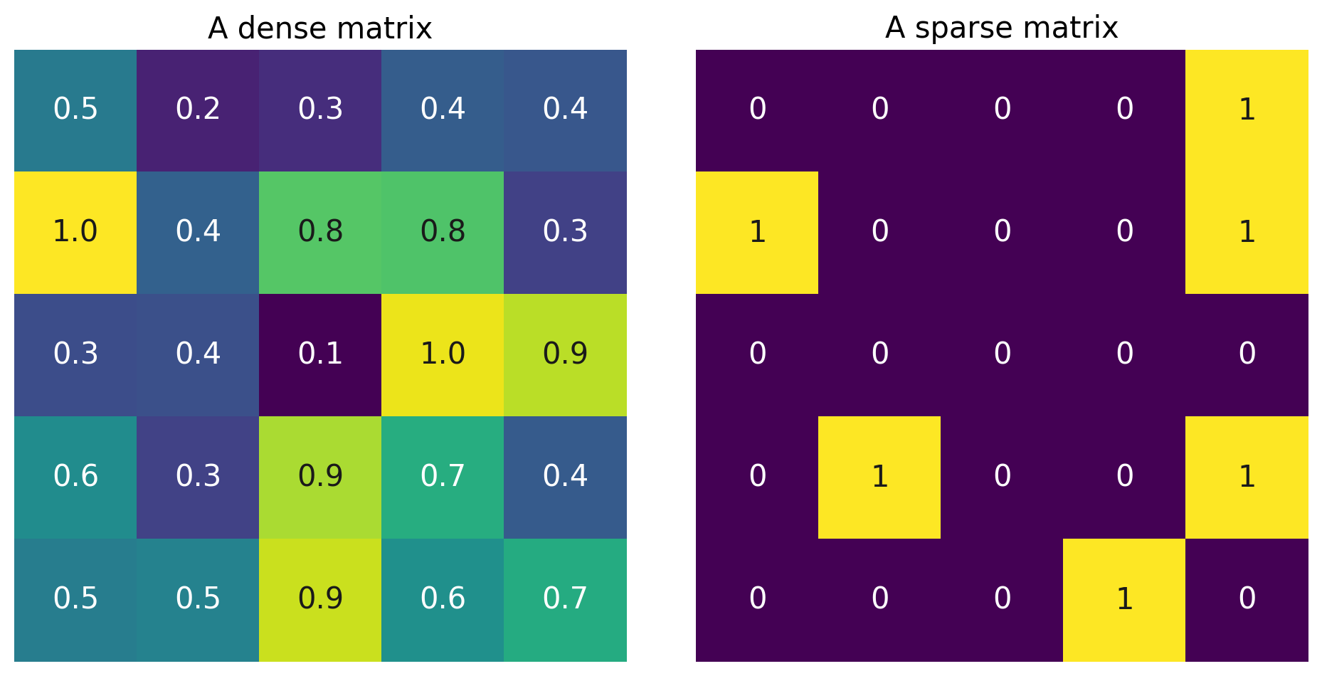
Larger L1 regularization leads to sparser solutions.

When is it OK to assume that the parameter vector is sparse? Whenever it is true that most features don’t affect the outcome. One use-case might be decoding low-level visual features from whole-brain fMRI: we may expect only voxels in V1 and thalamus should be used in the prediction.

WARNING: be careful when interpreting \(\theta\). Never interpret the nonzero coefficients as evidence that only those voxels/neurons/features carry information about the outcome. This is a product of our regularization scheme, and thus our prior assumption that the solution is sparse. Other regularization types or models may find very distributed relationships across the brain. Never use a model as evidence for a phenomena when that phenomena is encoded in the assumptions of the model.

Exercise 6: Final evaluation on test data#

A) You can also use your cross-validation scores to choose the type of regularization! Based on ridge_validation_r2s and lasso_validation_r2s - what model would you select? Which type of regularization (if any) and what would the value of alpha be?

YOUR ANSWER HERE

B) Now we want to report our model of choice’s performance on the completely held-out test data. Note we didn’t use this test data for any model selection!

Grab the correct model based on your answer to A and report the R2 score of the predictions on the test data.

Remember that you stored your models in the ridge_models and lasso_models dictionary where the key is the alpha value. So you should be able to retrieve the Rdige model with alpha 1 as ridge_models[1] for example

# your code here

Note that we could have done an even more comprehensive search and used both ridge and lasso regularization, changing the weights of each! This would be a grid search over hyperparameters (as we’d try every combo of Lasso alpha and Ridge alpha in a grid-like pattern). We won’t do this for time but sklearn’s ElasticNet (https://scikit-learn.org/stable/modules/generated/sklearn.linear_model.ElasticNet.html) allows you to fit a linear regression model with both types of regularization.

Mathematical Tools for Neuroscientists

Tutorial 2

Contents