Tutorial 1
Contents
![]()
Tutorial 1#
Probability & Statistics III: Statistical Encoding & Decoding
[insert your name]
Important reminders: Before starting, click “File -> Save a copy in Drive”. Produce a pdf for submission by “File -> Print” and then choose “Save to PDF”.
To complete this tutorial, you should have watched Video 8.1 and 8.2.
Imports
# @markdown Imports

# Imports
import numpy as np
import matplotlib.pyplot as plt
import ipywidgets as widgets  # interactive display
import math
Plotting functions
# @markdown Plotting functions
import numpy
from numpy.linalg import inv, eig
from math import ceil
from matplotlib import pyplot, ticker, get_backend, rc
from mpl_toolkits.mplot3d import Axes3D
from itertools import cycle


%config InlineBackend.figure_format = 'retina'
plt.style.use("https://raw.githubusercontent.com/NeuromatchAcademy/course-content/master/nma.mplstyle")
Helper functions
# @markdown Helper functions
def twoD_Gaussian(xdata_tuple, amplitude, xo, yo, sigma_x, sigma_y, theta, offset):
  """Create 2D Gaussian based on parameters

  Args:
    xdata_tuple (ndarray): grid of x and y values to compute Gaussian for
    amplitude (scalar): amplitude of Gaussian
    xo (scalar): center of Gaussian in x coordinates
    yo (scalar): center of Gaussian in y coordinates
    sigma_x (scalar): standard deviation of Gaussian in x direction
    sigma_y (scalar): standard deviation of Gaussian in y direction
    theta (scalar): rotation angle of Gaussian
    offset (scalar): offset of all Gaussian values

  Returns:
    ndarray: Gaussian values at every x/y point

  """
  (x, y) = xdata_tuple
  xo = float(xo)
  yo = float(yo)
  a = (np.cos(theta)**2)/(2*sigma_x**2) + (np.sin(theta)**2)/(2*sigma_y**2)
  b = -(np.sin(2*theta))/(4*sigma_x**2) + (np.sin(2*theta))/(4*sigma_y**2)
  c = (np.sin(theta)**2)/(2*sigma_x**2) + (np.cos(theta)**2)/(2*sigma_y**2)
  g = offset + amplitude*np.exp( - (a*((x-xo)**2) + 2*b*(x-xo)*(y-yo)+c*((y-yo)**2)))
  return g.ravel()
The data#
In this tutorial, we will be working with simulated neural data from a visual neuron in response to Gaussian white noise and MNIST images (we’ll call these natural scenes for ease even though they aren’t very natural). We will be fitting LNP models for both types of stimuli separately. We have 10000 images for each type of stimuli and each image is 10 x 10 pixels.
The next cell gives you WN_images and NS_images, the white noise and MNIST images respectively. Each is 10000 x 100 so the images have already been vectorized.
Execute this cell to get and visualize example image of each type (may take a few min to download)
# @markdown Execute this cell to get and visualize example image of each type (may take a few min to download)

np.random.seed(123)
n_images = 10000

# Get WN images
WN_images = np.random.randn(n_images, 10*10)

# Get NS images
from sklearn.datasets import fetch_openml
mnist = fetch_openml(name='mnist_784')
mnist_images = np.array(mnist.data)
mnist_images = mnist_images/255
mnist_images = mnist_images - np.mean(mnist_images)

mnist_images = mnist_images.reshape((-1, 28, 28))[:, 4:24, 4:24]
mnist_images = mnist_images[:, ::2, ::2]
NS_images = mnist_images[:n_images].reshape((-1, 10*10))

fig, axes = plt.subplots(1, 2, figsize=(10, 5))
axes[0].imshow(WN_images[0].reshape((10, 10)), vmin=-1, vmax=1, cmap='gray')
axes[1].imshow(NS_images[0].reshape((10, 10)), vmin=-1, vmax=1, cmap='gray')
axes[0].axis('Off')
axes[1].axis('Off')
axes[0].set(title='WN example image')
axes[1].set(title='NS example image');
---------------------------------------------------------------------------
ModuleNotFoundError                       Traceback (most recent call last)
Cell In[4], line 10
      7 WN_images = np.random.randn(n_images, 10*10)
      9 # Get NS images
---> 10 from sklearn.datasets import fetch_openml
     11 mnist = fetch_openml(name='mnist_784')
     12 mnist_images = np.array(mnist.data)

ModuleNotFoundError: No module named 'sklearn'
The response to each image is a summed spike count response so we do not have to worry about accounting for the time lags of the stimuli etc. We are simulating the neuron as an LNP model with an exponential nonlinearity so a linear filter, then exponential, then Poisson draws. Note that this means our LNP fits will be really good because we are using the correct model (this will literally never happen in real life…)
Execute the next cell to simulate our neuron and get WN_spike_counts and NS_spike_counts. filter is the true linear filter of this neuron.
Execute to simulate neural responses
# @markdown Execute to simulate neural responses
np.random.seed(0)

x = np.arange(-5, 5, 1)
y = np.arange(-5, 5, 1)
x, y = np.meshgrid(x, y)

sd_x = 1.4
sd_y = .5
gauss = twoD_Gaussian((x,y), 1, 0, 0, sd_x, sd_y, 35, 0)
filter = gauss.reshape((10, 10))

WN_lambda = np.exp(np.dot(WN_images, filter.reshape((-1,))))
WN_spike_counts = np.random.poisson(WN_lambda)

NS_lambda = np.exp(np.dot(NS_images, filter.reshape((-1,))))
NS_spike_counts = np.random.poisson(NS_lambda)

fig, axes = plt.subplots(1, 2, figsize=(10, 5), sharex=True)
axes[0].plot(WN_spike_counts[0:100], 'ok')
axes[1].plot(NS_spike_counts[0:100], 'ok')
axes[0].set(ylabel='Spike counts', xlabel='Image number', title='WN')
axes[1].set(xlabel='Image number', title='NS');
---------------------------------------------------------------------------
NameError                                 Traceback (most recent call last)
Cell In[5], line 16
     13 WN_lambda = np.exp(np.dot(WN_images, filter.reshape((-1,))))
     14 WN_spike_counts = np.random.poisson(WN_lambda)
---> 16 NS_lambda = np.exp(np.dot(NS_images, filter.reshape((-1,))))
     17 NS_spike_counts = np.random.poisson(NS_lambda)
     19 fig, axes = plt.subplots(1, 2, figsize=(10, 5), sharex=True)

NameError: name 'NS_images' is not defined
Exercise 1: Computing an STA#
We want to fit an LNP model for each type of stimulus. Since our white noise is stochastic and spherically distributed, we know we can compute a spike triggered average and it will be an unbiased estimator for our linear filter. In fact, we will assume an exponential nonlinearity so it will be the maximum likelihood estimator for our linear filter.
Fill out the code below to create a function that computes the STA from a set of images and associated spike counts. Compute this STA for both white noise and natural scenes. Run the next cell to visualize your computed STAs next to the original (true) linear filter.
Answer#
Fill out code below
WN_spike_counts.shape
(10000,)
def compute_STA(images, spike_counts):

  STA = ...

  return STA


WN_STA = ...
NS_STA = ...
Execute to visualize your computed STAs and the original filter
# @markdown Execute to visualize your computed STAs and the original filter

fig, axes = plt.subplots(1, 3, figsize=(15, 5))

axes[0].imshow(filter.reshape((10, 10)), vmin=-1, vmax=1, cmap='gray')
axes[1].imshow(WN_STA.reshape((10, 10)), vmin=-1, vmax=1, cmap='gray')
axes[2].imshow(NS_STA.reshape((10, 10)), vmin=-1, vmax=1, cmap='gray')

for i in range(3):
  axes[i].axis('Off')

axes[0].set(title='True filter')
axes[1].set(title='White noise STA')
axes[2].set(title='Natural scenes STA');
---------------------------------------------------------------------------
AttributeError                            Traceback (most recent call last)
Cell In[8], line 6
      3 fig, axes = plt.subplots(1, 3, figsize=(15, 5))
      5 axes[0].imshow(filter.reshape((10, 10)), vmin=-1, vmax=1, cmap='gray')
----> 6 axes[1].imshow(WN_STA.reshape((10, 10)), vmin=-1, vmax=1, cmap='gray')
      7 axes[2].imshow(NS_STA.reshape((10, 10)), vmin=-1, vmax=1, cmap='gray')
      9 for i in range(3):

AttributeError: 'ellipsis' object has no attribute 'reshape'
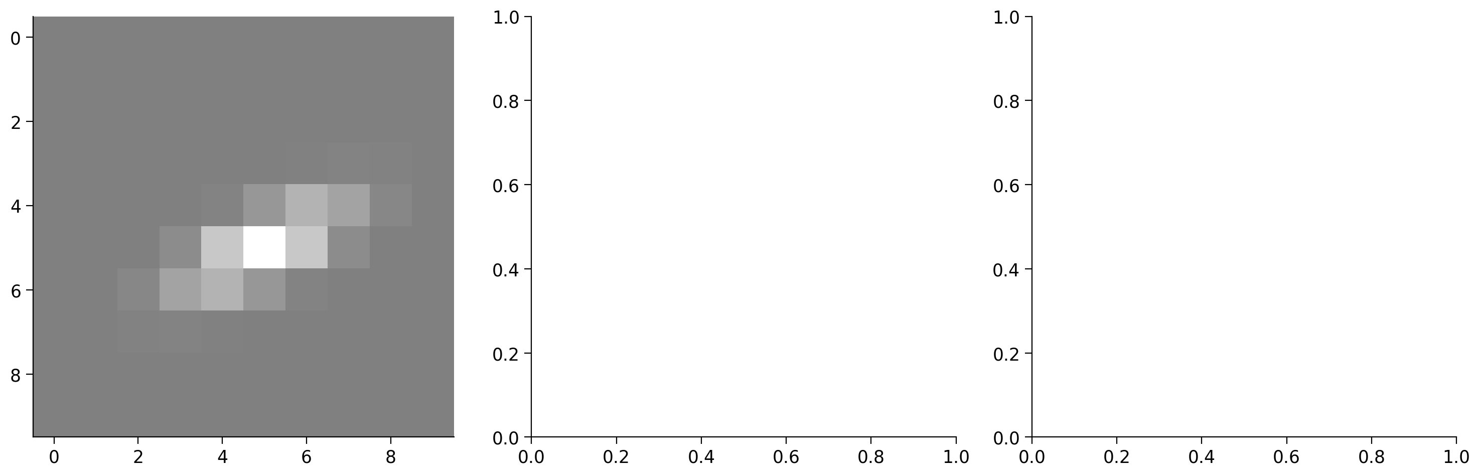
Note that the white noise STA is a pretty good estimate for the true filter, but the natural scenes STA is not!
(Optional) Exercise: Estimate the nonlinearity#
Estimate the nonlinearity of the LNP model (so no longer predefine it as exponential) using the method discussed in Video 8.2.
Exercise 2: Numerically finding the filter with natural scenes data#
The STA was a very convenient estimate of our linear filter of an LNP model for the white noise stimuli. Unfortunately, it is a bad estimator for the natural scenes stimuli so we will have to use a numerical approach to estimate the filter using this data. In this exercise, we will implement gradient descent ourselves.
A) Negative log likelihood equation#
To implement gradient descent ourselves, we will need to compute the derivative of the negative log likelihood.
Write out the negative log likelihood equation for our LNP model with an exponential nonlinearity. Simplify as much as possible. Drop constants that don’t depend on the filter (so we won’t compute the true NLL but the relative NLL for different filters). Show the math! Use y for the spike counts and x for the images.
Make the final equation clear either with the green text below or by putting it in a box or otherwise highlighting it.
Answer#
Put NLL = … equation here (show work above or below)
B) Negative log likelihood computation#
Use your equation in part A to fill out the code below to compute the negative log likelihood for a given filter (k) and set of images (x) and spike counts (y). x and y would be the same shape as WN_images and WN_spike_counts for example
Answer#
Fill out code below
def compute_NLL(k, x, y):

    NLL = ...

    return NLL

fake_k = np.zeros((100,))
NLL = compute_NLL(fake_k, WN_images, WN_spike_counts)
print(NLL)
Ellipsis
C) Compute dNLL/dk#
Take your answer in part A and now take the derivative with respect to \(\bar{k}\). Note that \(\bar{k}\) is a vector so this can get tricky! I would take the derivative with respect to \(\bar{k}_o\) first (the first element of \(k\)). Since each entry of \(\bar{k}\) is present in the negative log likelihood equation in a similar manner, you should be able to extend your calculation for \(\frac{dNLL}{d\bar{k}_0}\) to figure out the whole vector \(\frac{dNLL}{d\bar{k}}\).
When in confusion about dot products, my recommendation is to write out the first few elements of the dot product computation for clarifiation.
Make the final equation clear either with the green text below or by putting it in a box or otherwise highlighting it. Show your work!
Answer#
Put dNLL/dk = … equation here (show work above or below)
D) Implementing gradient descent#
We now have all the tools we need to implement gradient descent to find an estimate of our filter k using the natural scenes data.
Fill out the following code to perform gradient descent and then call it for the natural scenes data. The following cells plot the loss function (negative log likelihood) over step of the gradient descent algorithm and the fitted filter.
Answer#
Fill out code below
Execute to visualize negative log likelihood over gradient descent
def gradient_descent(x, y, init_guess, n_steps = 500, alpha=10**-6):

    k = init_guess
    NLL = np.zeros((n_steps,))
    for i_step in range(n_steps):

      # Update estimate of k (assign as k)
      # your code here

      # Compute NLL at each step
      NLL[i_step] = compute_NLL(k, x, y)

    return k, NLL

k, NLL = ...
---------------------------------------------------------------------------
TypeError                                 Traceback (most recent call last)
Cell In[10], line 15
     11       NLL[i_step] = compute_NLL(k, x, y)
     13     return k, NLL
---> 15 k, NLL = ...

TypeError: cannot unpack non-iterable ellipsis object
Execute to visualize your estimated filter
# @markdown Execute to visualize negative log likelihood over gradient descent
fig, axes = plt.subplots()
axes.plot(NLL,'-ok')
axes.set(ylabel='NLL', xlabel='Gradient descent step', title='LNP fitting');
---------------------------------------------------------------------------
TypeError                                 Traceback (most recent call last)
Cell In[11], line 3
      1 # @markdown Execute to visualize negative log likelihood over gradient descent
      2 fig, axes = plt.subplots()
----> 3 axes.plot(NLL,'-ok')
      4 axes.set(ylabel='NLL', xlabel='Gradient descent step', title='LNP fitting');

File /opt/hostedtoolcache/Python/3.8.14/x64/lib/python3.8/site-packages/matplotlib/axes/_axes.py:1664, in Axes.plot(self, scalex, scaley, data, *args, **kwargs)
   1662 lines = [*self._get_lines(*args, data=data, **kwargs)]
   1663 for line in lines:
-> 1664     self.add_line(line)
   1665 if scalex:
   1666     self._request_autoscale_view("x")

File /opt/hostedtoolcache/Python/3.8.14/x64/lib/python3.8/site-packages/matplotlib/axes/_base.py:2340, in _AxesBase.add_line(self, line)
   2337 if line.get_clip_path() is None:
   2338     line.set_clip_path(self.patch)
-> 2340 self._update_line_limits(line)
   2341 if not line.get_label():
   2342     line.set_label(f'_child{len(self._children)}')

File /opt/hostedtoolcache/Python/3.8.14/x64/lib/python3.8/site-packages/matplotlib/axes/_base.py:2363, in _AxesBase._update_line_limits(self, line)
   2359 def _update_line_limits(self, line):
   2360     """
   2361     Figures out the data limit of the given line, updating self.dataLim.
   2362     """
-> 2363     path = line.get_path()
   2364     if path.vertices.size == 0:
   2365         return

File /opt/hostedtoolcache/Python/3.8.14/x64/lib/python3.8/site-packages/matplotlib/lines.py:1031, in Line2D.get_path(self)
   1029 """Return the `~matplotlib.path.Path` associated with this line."""
   1030 if self._invalidy or self._invalidx:
-> 1031     self.recache()
   1032 return self._path

File /opt/hostedtoolcache/Python/3.8.14/x64/lib/python3.8/site-packages/matplotlib/lines.py:664, in Line2D.recache(self, always)
    662 if always or self._invalidy:
    663     yconv = self.convert_yunits(self._yorig)
--> 664     y = _to_unmasked_float_array(yconv).ravel()
    665 else:
    666     y = self._y

File /opt/hostedtoolcache/Python/3.8.14/x64/lib/python3.8/site-packages/matplotlib/cbook/__init__.py:1369, in _to_unmasked_float_array(x)
   1367     return np.ma.asarray(x, float).filled(np.nan)
   1368 else:
-> 1369     return np.asarray(x, float)

TypeError: float() argument must be a string or a number, not 'ellipsis'
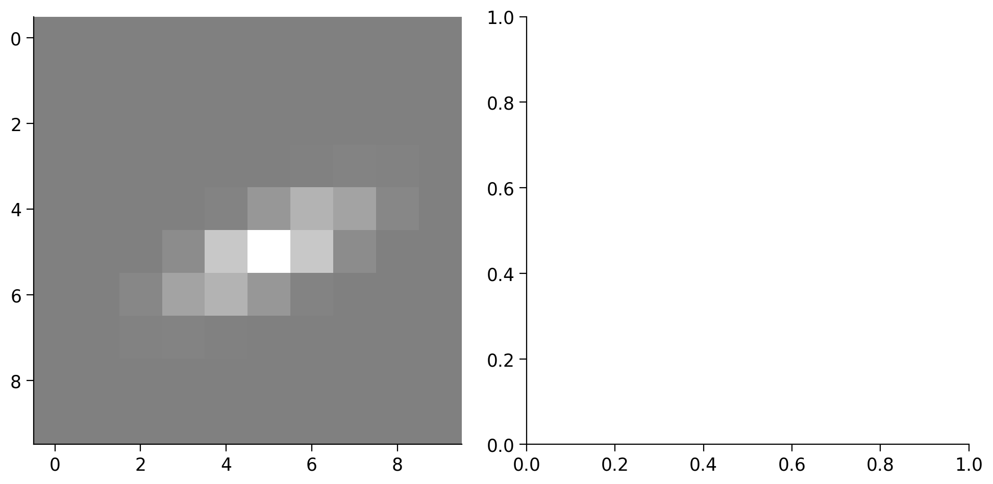
# @markdown Execute to visualize your estimated filter

fig, axes = plt.subplots(1, 2, figsize=(10, 5))

axes[0].imshow(filter.reshape((10, 10)), vmin=-1, vmax=1, cmap='gray')
axes[1].imshow(k.reshape((10, 10)), vmin=-1, vmax=1, cmap='gray')

for i in range(2):
  axes[i].axis('Off')

axes[0].set(title='True filter')
axes[1].set(title='Estimate of k using NS data');
---------------------------------------------------------------------------
NameError                                 Traceback (most recent call last)
Cell In[12], line 6
      3 fig, axes = plt.subplots(1, 2, figsize=(10, 5))
      5 axes[0].imshow(filter.reshape((10, 10)), vmin=-1, vmax=1, cmap='gray')
----> 6 axes[1].imshow(k.reshape((10, 10)), vmin=-1, vmax=1, cmap='gray')
      8 for i in range(2):
      9   axes[i].axis('Off')

NameError: name 'k' is not defined
E) Larger steps#
In the next cell, try out performing gradient descent using your function above and step size alpha = \(10^{-5}\) instead of \(10^{-6}\). What happens with the negative log likelihood over time? Why is this happening?
k, NLL = ...

fig, axes = plt.subplots()
axes.plot(NLL,'-ok')
axes.set(ylabel='NLL', xlabel='Gradient descent step', title='LNP fitting');
---------------------------------------------------------------------------
TypeError                                 Traceback (most recent call last)
Cell In[13], line 1
----> 1 k, NLL = ...
      3 fig, axes = plt.subplots()
      4 axes.plot(NLL,'-ok')

TypeError: cannot unpack non-iterable ellipsis object
Answer#
Text answer here
Extra info#
We didn’t need to compute gradient descent ourselves. We could have used an optimizer from scipy as shown in the following code. We computed our gradient by hand for practice and to really look “under the hood” of gradient descent.
from scipy.optimize import minimize
init_guess = np.zeros((10*10,))
outs = minimize(compute_NLL, init_guess, (NS_images, NS_spike_counts))


plt.imshow(outs.x.reshape((10, 10)), vmin=-1, vmax=1,cmap='gray')
plt.axis('Off');
---------------------------------------------------------------------------
NameError                                 Traceback (most recent call last)
Cell In[14], line 3
      1 from scipy.optimize import minimize
      2 init_guess = np.zeros((10*10,))
----> 3 outs = minimize(compute_NLL, init_guess, (NS_images, NS_spike_counts))
      6 plt.imshow(outs.x.reshape((10, 10)), vmin=-1, vmax=1,cmap='gray')
      7 plt.axis('Off');

NameError: name 'NS_images' is not defined